The Fan Approximation
Contents
- Prerequisites
- Original Fan Approximation
- Fan Approximation and Unit Commitment
- Revised Fan Approximation
- Vector Names in PLEXOS
- Non-convex Marginal Cost Functions
- Numerical Example
- References
1. Prerequisites
Fuel offtake (f) is expressed as a polynomial function of power generation (p) thus:
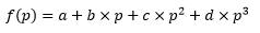 Where
Where
- p is generator power
- a is the zero-order (constant) term
- b is the first-order (linear) term
- c is the second-order (quadratic) term
- d is the third-order (cubic) term
a is referred to as 'no-load' offtake.
Power can be produced between a minimum level (Pmin) and maximum (Pmax).
The orthodox linear representation for this non-linear function uses separable programming that divides the x-axis into tranches so that:

The separable programming assumption is that the tranche incremental 'cost' coefficients are monotonically non-decreasing. If this were not the case the fuel offtake would be understated since lowest cost tranches are 'cleared' first. In the case where this convexity assumption is violated, integer variable can be introduced to force clearing of the tranches in nominal order rather than cost order.
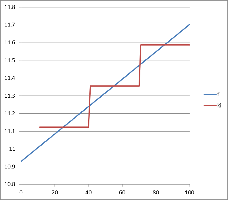
In most real applications that fuel function is very close to linear, and so the piecewise linear approximation is highly accurate. However, in pricing the approximation is less attractive as shown here, where we plot the marginal cost from the derivative of the cost function versus the stepwise incremental cost function of the approximation:
This stepwise pricing function is unavoidable but the original Fan Approximation seeks to address limitations of this model when spare capacity (for use as spinning or regulation reserves) is to be co-optimised with energy (power):
Firstly the standard piecewise linear model does not represent spare capacity directly, though it can be calculated as:

And secondly when unit commitment (on/off) decisions are considered in combination with spare capacity for reserve, the relaxation of this model tends to be poor, with the relaxation often having generators 'on' and providing technically infeasible amounts of reserve e.g. a generator running at notional 'zero' load in order to provide Pmax level of spare capacity.
Given that spare capacity is a fundamental element of an energy-reserve co-optimisation it is convenient, and potentially more efficient, to include it directly in the cost function, hence the Fan Approximation.
2. Original Fan Approximation
The Fan Approximation is an alternative separable programming approach to modelling the polynomial cost function in a linear optimisation. The Fan Approximation was first described by [1]. The model considers the 2-dimensional space of energy and spare capacity directly, and divides this space into 'fans' (analogous to tranches in the traditional model).
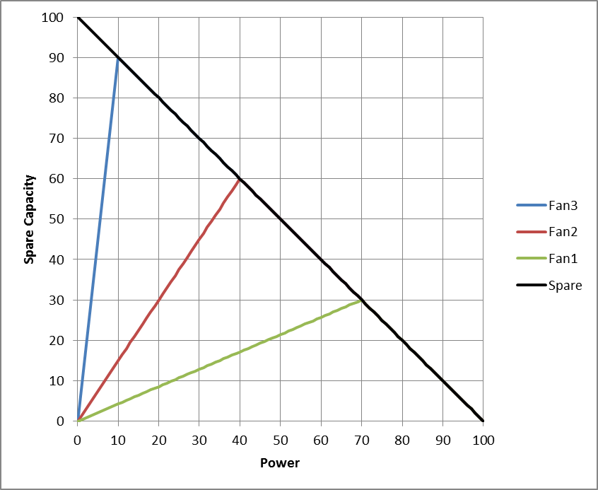
Each fan of the model is bounded by a 'reference ray' running from the origin at a slope described by the ratio of incremental spare capacity in the fan to power. For example, the first fan (green line) is defined as the ratio 30/70, while the second has a slope of 40/60, which is an incremental slope (over of the first fan) of 40/60 - 30/70 = 10/42.
- The single power variable p carries a cost term (k0) equal to the average value of the polynomial function between zero and Pmax.
- The fan variables (si) carry cost terms (ki) representing the change in cost as power is substituted by spare capacity.
The term pi refers to the power corresponding to the intersection of the reference ray for fan i and the capacity line (45-degree line).
The complete formulation is thus:
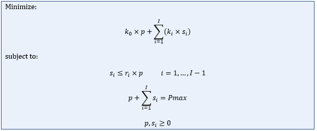
The first constraint is called the 'reference ray' constraint, the second is the maximum capacity constraint
3. Fan Approximation and Unit Commitment
We introduce unit commitment to the Fan Approximation by including the variable n being the binary on/off state of the unit:

In addition we can improve the linear relaxation of this problem by introducing the following constraint:

This constraint eliminates solutions where the generator is committed 'on' but with all capacity spare. It is known as the 'bath tub' constraint because it creates a feasible region the shape of an inverted bath tub.
4. Revised Fan Approximation
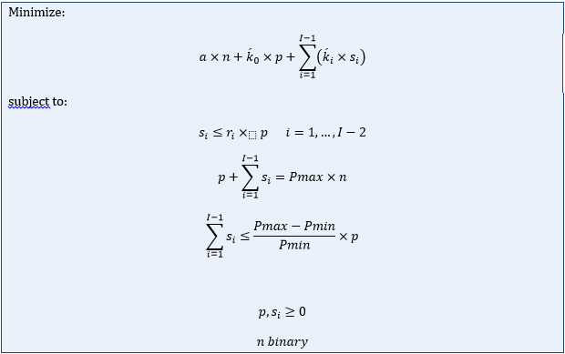
The Revised Fan Approximation (RFA) seeks to improve the performance of the original Fan Approximation for the co-optimisation of unit commitment with energy and reserve by including the commitment variable in the cost function in place of the Ith fan. The commitment variable carries the cost term of a (the no-load cost), and the last fan is dropped from the formulation, as is the last (I - 1) reference ray constraint.
The cost terms for p and si terms are now based on a modified polynomial cost function that excludes the constant term:

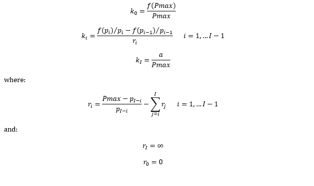
Hence these equations apply:

kI is no longer necessary
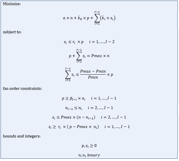
And the revised formulation is:
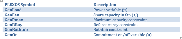
5. Vector Names in PLEXOS
The following names are used in PLEXOS for the variable components of this formulation:
6. Non-convex Marginal Cost Functions
The notional knowledge of a 3rd order polynomial approximation of the fuel offtake function leads to a potential non-convex continuous function if the second order derivative becomes zero above the minimum operational range. The linear programming approximation could then involve non-monotonically increasing incremental tranches. The logical lowest to highest clearing is no longer possible since the incremental stepwise function has non-increasing consecutive tranches. In order to solve non-convex functions using linear programming, auxiliary integer variables are required to clear the objective function tranches in the correct order, even when the decreasing successive incremental costs exists. The following formulation is then required.
The different generation levels require the activation of the integer variables ni. It is easy to deduce that the incremental order is imposed by n(i-1)≥ni constraint. Two additional constraints are also required for defining each tranche length: each fan variable has an upper limit of zero if the unit is either offline or the previous tranche is active; if the current tranche is not active, the fan variable must be greater than zero (spare capacity is available).
7. Numerical Example
Assume a thermal generator with the following technical characteristics:
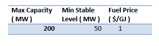
Now assume the following heat rate data:
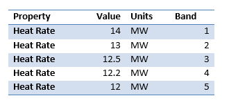
The fuel offtake function will look like the figure (a). In figure (b) the piecewise linear approximation of the offtake cubic approximation, considering the slope as linear interpolation of evenly distributed segments (or tranches) across the operational range (i.e. Between Pmax and MSL).
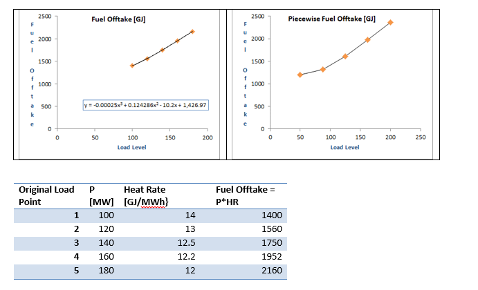
From the 3rd order polynomial fit to the 5 fuel offtake defined points, the no-load cost (or heat base since Price=1) is the intercept of the offtake function i.e. a=1,426.97. Considering the RFA description above, the fuel offtake function F' is simply computed by: evaluating the polynomial fit into evenly distributed operational points and subtracting "a" from the total offtake.
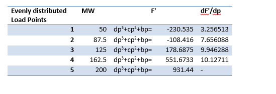
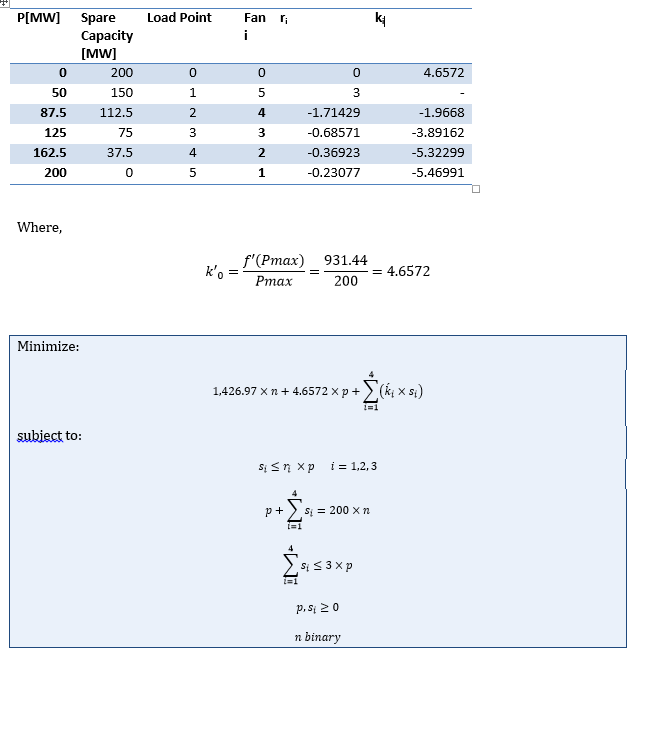
The fan approximation creates the equivalent incremental cost function (dF'/dp column) using the spare capacity values. In this example, 4 fan variables "s" will be required. The RFA parameters are computed as follows:
8. References
[1] G.R. DRAYTON. Coordinating Energy and Reserves in a Wholesale Electricity Market, Doctoral Thesis, University of Canterbury, New Zealand. 1997.