Graph Layout
Contents
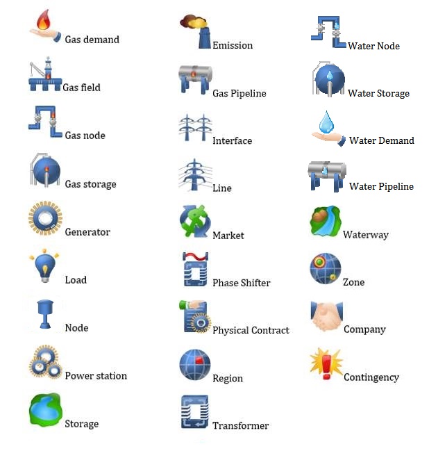
Convention: any visual entity which is put on the graph and represents a PLEXOS object is referred to as a pin object.
1. Input Graph Layout
This chapter introduces graph style visualization functions of PLEXOS GUI for input databases.
1.1. Access to the Graph Window
Graph window is accessed using the Graph button from the Graph tab of ribbon-style menu
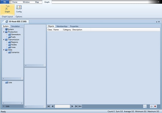
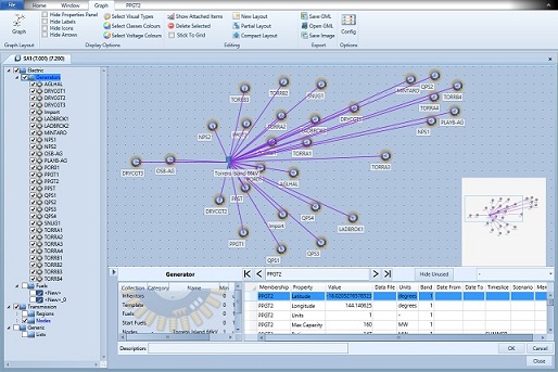
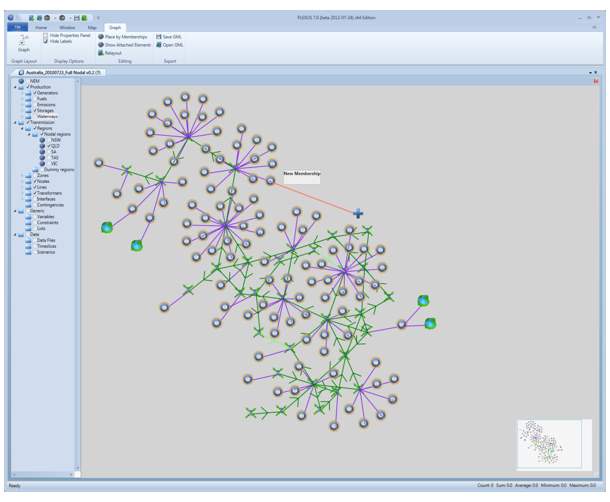
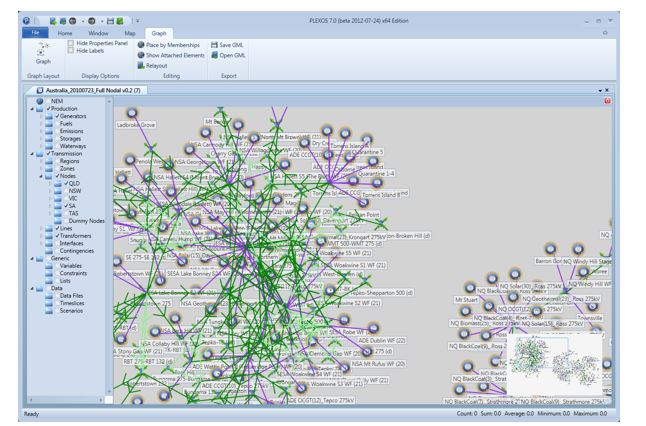
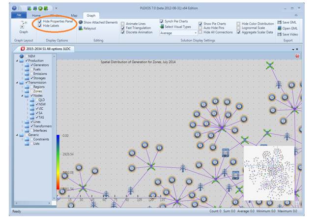
1.2. Graph Window Layout
The graph window has four parts:
- Tree of filters on the left
- Graph area with visualized objects
- Mini-map (bottom-right corner)
- Property pane (when visible)
Most of the other controls are located on the Graph tab of the ribbon style menu.
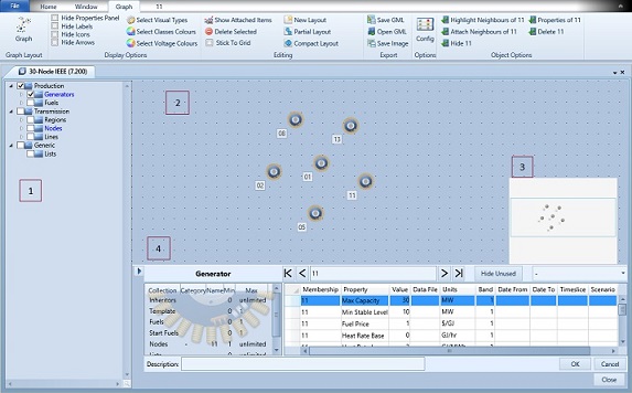
1.3. Tree of Filters
Objects can be put to or removed from the graph by checking or unchecking corresponding filters. Enabling a filter makes all objects associated via memberships also visible, the corresponding nodes on the tree are checked as well. For example: when we enable some fuel filter on the tree, this will enable all the generators which use that fuel. Disabling the fuels will uncheck all the filters and remove the associated objects from the Graph.
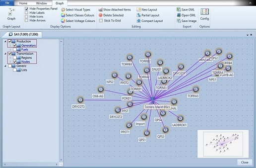
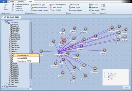
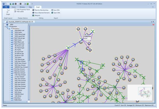
When a particular node is double-clicked, it's icon on the graph is highlighted orange. Right-clicking the graph returns the highlighted icon to its normal state. Double-click on tree node also centres the graph about that object (provided that the object is checked).
The user can also use the right-click menu on the tree object nodes and highlight, delete or examine the properties of each object.
1.4. Graph Controls
The graph can be repositioned by left clicking and dragging the graph area or dragging the viewing area in the mini-map.
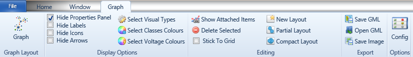
Display Options Group
Hide Properties Panel: Hides/displays the property pane for a selected element at the bottom or right of the graph.The property pane can also be shown if the user double-clicks an object on the graph or presses F4 while hovering the mouse over the pin icon, i.e. F4 works like a toggle, it turns the property page on and off. When the property pane is open, left-clicking on a pin icon will refresh the property pane with the pins updated properties.
Hide Labels: Hides labels with objects names.
Hide Icons: Option collapses pins icons to small grey dots, regular icon appears when mouse pointer hovers over the pin and collapses back when mouse leaves that pin
Hide Arrows: " Option removes arrows from all of the lines
Select Classes Colours: User can select colour for each transportation class of objects (Line, Transformer, Waterway, Gas Pipeline or Water Pipeline). This selection is saved and applies to all visualization layouts
Select Voltage Colours: User can select colour for each value of voltage of Lines and Transformers. Also, user can select level of significant voltage ("High Voltage"), so that lines and transformers with voltage equal or above that level will have thicker lines. This selection is saved and applies to all visualization layouts
Select Visual Types: Setting the type of visualization (pin, line or area) for each class. Any object can be visualized as a pin object; Line, Transformer, Waterway, Gas Pipeline, and Water Pipeline objects can be visualized as lines; Zone, Region, Interface, Contingency, Gas Zone and Water Zone objects can be visualized as area objects.
All classes added as pin objects will have its associated collection folder, within the graph view object tree, coloured blue. Please note that the graph view object tree colouring scheme behaves differently to the regular input object tree.
Default view of a property page, clicking the arrow at the top left corner of the property pane toggles between positioning it on the right edge or bottom of the window.
Editing Group
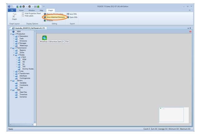
Show Attached Elements: Puts all the objects which have memberships with currently selected objects into view.
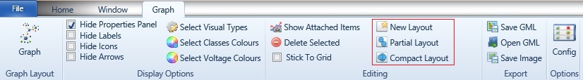
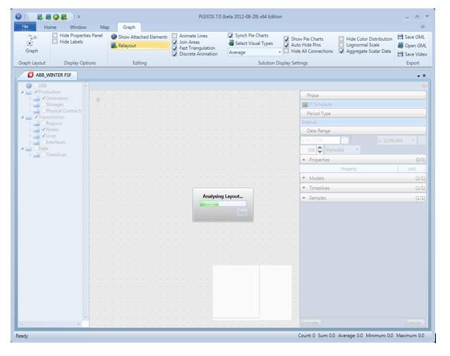
New Layout: Starts automatic layout process.
Partial Layout: Starts automatic layout process for the objects of current layout which weren't positioned manually, or are not selected/highlighted.
Compact Layout: Shrinks layout area to the size of objects network.
Delete Selected: Deletes all selected pin items from database.
Stick To Grid: Positions of pin objects are set to the nearest grid node.
Export Group
Save Image: Saves current Graph view as .png image file.
Save GML: Saves currently shown Graph as .gml file.
Open GML: Loads objects mutual positions from the selected .gml file.
The Legend of line colours on the graph are as follows:
- Line: Green
- Transformer: Light Green
- Waterway: Blue
- Gas Pipeline: Cadet Blue
- Water Pipeline: Deep Sky Blue
- Membership: Violet
- Inherited Membership: Magenta
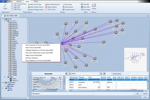
Right-click Menu of Pin Objects
Show Properties: Opens the property pane for the pin objects
Highlight Neighbours: Highlights objects connected via memberships to the pin object\\ Add New ...: Opens a create object dialog box. The type of new object is defined by what is selected on the tree of filters (on the picture above Generators node is selected, so that the option reads as "Add New Generator"). If more than one type of collection can be established, collection type selection dialog is open and the user can select the desired type.
Right-click menu of memberships, lines, gas pipelines, water pipeline, transformers and waterways
Line Name: Displays the name and type of line selected, i.e. whether it is a membership or water line for example. The property pane of the underlying PLEXOS object will open.
Edit Line: Places the line into 'Edit Mode'.
Delete Line: Deletes the selected object.
It is not possible to edit or delete inherited memberships between objects.
1.5. Manual Positioning
Pins can be arranged manually by dragging them to the desired positions, alternatively the automatic layout option (uses force-driven layout algorithm) is available. Automatic layout works with enabled objects.
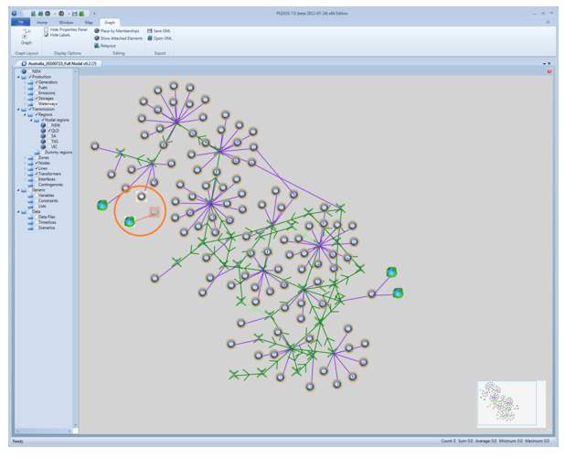
New pin objects can be added by pointing on a desired location in the Graph and using the right-click menu.
New pin objects can be added by pointing on a desired location in the Graph and using the right-click menu.
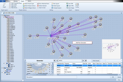
Selecting the Add New ... menu item will open new object dialog where the user can create the new object. After closing the new object dialog, the user can position the new object by left-clicking at a desired location.
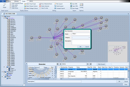
Setting up new objects
To recap, the user can create an object by right-clicking on any existing pin (the object is going to be created along with memberships with the clicked pin object) and selecting corresponding menu option. After that the new object dialog will open, where the user can put name, description and select category. In order to move any pin object manually user left-press on the object and then drag the it to the desired location. Pin selection is done by clicking on a pins icon. Multi-selection is done by holding the control key and left-clicking pin objects. Another option for multi pins selection is to draw a rectangle by pressing and holding left mouse button together with moving mouse pointer.
1.5.1. Creating Objects Represented via a Line
Lines, Waterways, Transformers, Gas Pipelines and Water Pipelines are created via the following steps:
- Highlight the class of object to be created e.g. Lines
- Select the object pins that will be connected via the new Lines by holding down the control key and left-click each pin in turn. The order of selection is important, if we want power to travel from Node 1 to Node 2 to Node 3 for instance, we must select them in that order.
- Right-click any selected object, Node 1, Node 2 or Node 3 in our example and select Add New Line
- A dialog box will open where you can fill in the name.
- Select OK, PLEXOS will automatically name the remaining newly created line objects <line_name>_0, <line_name>_1 etc. These can be renamed, if required.
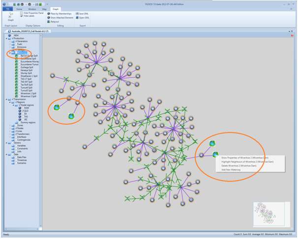
Waterway filter selected on the filter tree and four storages are highlighted on the graph. Richt-click Add New Waterway
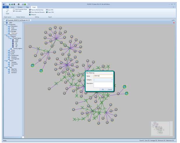
In the new object dialog the user can enters the waterways name <waterway_name>
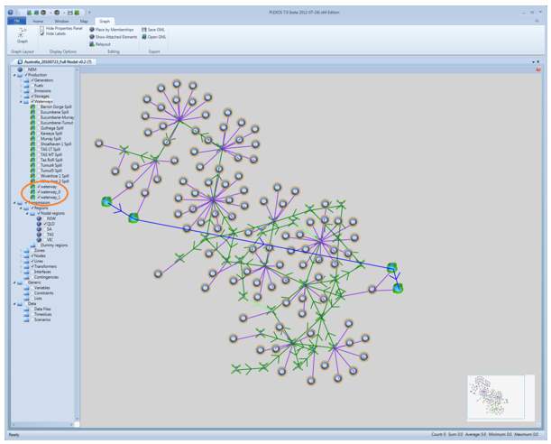
Created set of waterways, subsequent waterways are named <waterway_name>_0, <waterway_name>_1, etc.
Any existing membership can be changed by selecting the Edit line option from the corresponding line's context menu. As soon as line is in edit mode the user can reassign any pin object by holding the M-key and dragging the corresponding pin icon to another pin object.
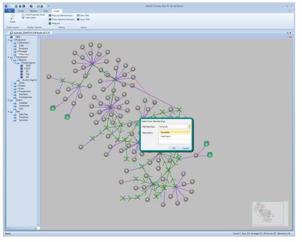
In order to create a new membership, hold the ''M-key and drag the pin icon from one pin object to the second pin object, representing both sides of the membership.
If selected pin objects can form multiple types of membership, select the desired type from the dialog box.
1.6. Automated Positioning
In order to make positioning of objects easier, the PLEXOS Graph window implements automatic object positioning functions.
Let's open database with no saved graph positions.
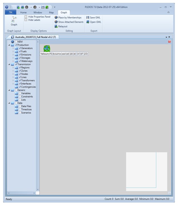
The convenient way is to arrange objects region by region.
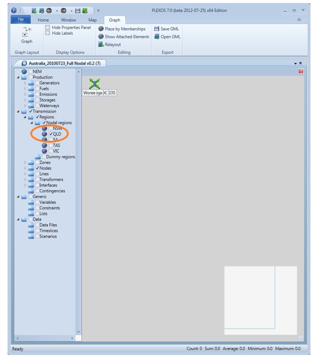
First region is selected
In order to be able to utilize the automated positioning algorithm we have to put all the connections and complementary objects for the selected set of nodes on the graph layout. To do so we can either enable all the corresponding filters on the filters tree manually, or use Show Attached Elements option from ribbon controls editing group.
We can call the Show Attached Elements option several times, to attach second order connections if required. As soon as all the objects we want to arrange within the region are selected, we call the Relayout function from the ribbon controls editing group.
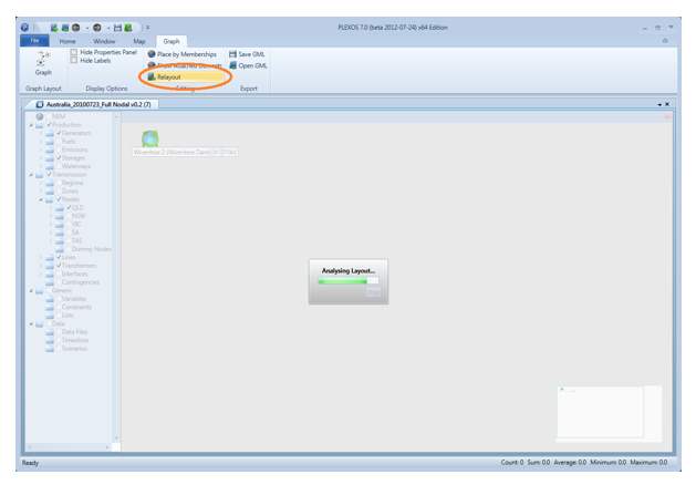
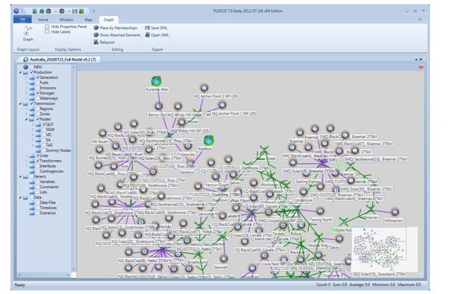
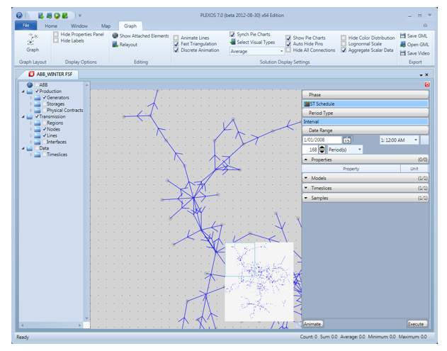
Automatic layout finished
After the first region is laid out, uncheck all filters and repeat procedure for a second region. When automatic layout is finished for the second region, we select all of its objects Control-key + A-key and drag the region to desired location.
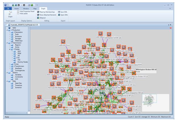
Second Region objects are selected
Both regions are positioned
This procedure can be repeated for multiple regions.
2. Solution Graph Layout
2.1. Data Viewer in Graph Style
The graph window is accessed using the Graph button from the Graph tab of ribbon-style menu
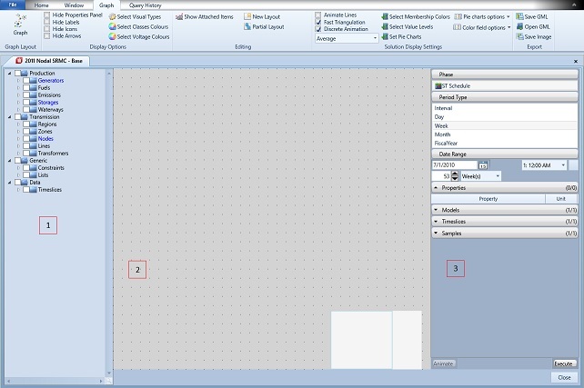
2.2. The graph window has three areas:
- Tree of filters: Organized in a tree with the same structure as the tree of objects in the main application.
- Graph area with visualized objects, mini-map (bottom-right corner) in the centre.
- Controls for selecting the property to visualize and setting up a query on the right.
Most of the other controls are located on the Graph tab of the ribbon style menu.
2.3. Tree of Filters
Objects can be put to or removed from the graph by checking or unchecking corresponding filters. Enabling a filter of objects displays all objects who share a membership to this filter objects on the graph, the corresponding nodes on the tree are also checked.
Exceptions are area objects which are represented as outlined areas of pin objects related to a chosen area object and line objects which are represented as a line connecting two pin objects related to a chosen line objects.
For example: when we enable some fuel filter on the tree, this will enable all the generators which use that fuel.
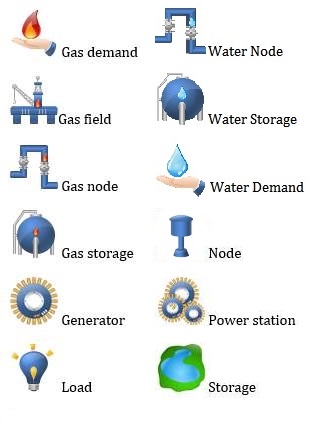
Currently only nodes, generators, storages, gas nodes, gas storages, water nodes, water storages, companies, loads, power stations, gas fields, gas demands, water demands, lines, transformers, gas pipelines, water pipelines and waterways can be visualized.
Disabling the fuels will uncheck all the filters and remove fuel and generator objects from the graph.
When a particular node is double-clicked it's icon on the graph is highlighted orange. Right-clicking the graph returns items to their normal state. Double-click on an object in tree also centres the graph about that object (provided that the object is checked)
2.4. Graph Controls

The graph can be repositioned by left clicking and dragging the graph area or dragging the viewing area in mini-map.
Display Options Group
Hide Properties: Hides/displays the solution execution section.
Hide Labels: Hides labels with objects names.
Hide Icons: Option collapses pins icons to small grey dots, regular icon appears when mouse pointer hovers over the pin and collapses back when mouse leaves that pin.
Hide Arrows: "Option removes arrows from all of the lines.
Select Classes Colours: User can select colour for each transportation class of objects (Line, Transformer, Waterway, Gas Pipeline or Water Pipeline). This selection is saved and applies to all visualization layouts.
Select Voltage Colours: User can select colour for each value of voltage of Lines and Transformers. Also, user can select level of significant voltage ("High Voltage"), so that lines and transformers with voltage equal or above that level will have thicker lines. This selection is saved and applies to all visualization layouts.
Select Visual Types: Setting the type of visualization (pin, line or area) for each class. Any object can be visualized as a pine object; Line, Transformer, Waterway, Gas Pipeline, Water Pipeline objects can be visualized as lines; Zone, Region, Interface and Contingency objects can be visualized as area objects.
All classes added as pin objects will have its associated collection folder, within the graph view object tree, coloured blue. Please note that the graph view object tree colouring scheme behaves differently to the regular input object tree.
Editing Group
Shows Attached Elements: Puts all the objects which have memberships with currently selected objects into view.
New Layout: Starts automatic layout process.
Partial Layout: Starts automatic layout process for the objects of current layout which weren't positioned manually, or are not selected/highlighted.
Solution Display Settings
Animate Lines: To indicate flow, animate the lines for demonstration purposes.
Fast Triangulation: Selects faster triangulation algorithm using Delaunay triangulation without creating regular grid and adding intermediate points.
Discrete Animation: Selects faster animation method without smoothing transitions and adding intermediate states.
Aggregation Mode: Combo box to select a method for managing combined values when objects are aggregated.
Average: Displays the average value of the aggregated objects.
Maximum: Displays the maximum value of the aggregated objects.
Minimum: Displays the minimum value of the aggregated objects.
Sum: Displays the summation of the aggregated objects.
Select Membership Colours: Opens a dialog for selecting custom colours of lines representing membership types.
Select Value Levels: Opens a dialog for selecting and adjusting value levels and colours for data colour fields.
Set Pie Charts: Opens a dialog for selecting and adjusting value levels and colours for pie charts.
Pie Chart Options: Combo box.
Synch Pie Charts: Updates values for pie charts after execution (see Execution section).
Show Pie Chart: Displays pie charts.
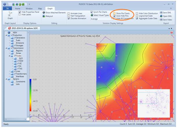
Auto Hide Pins: Filtered pins icons are only visible when mouse hovers over a point.
Colour Field Options: Combo box.
Hide Colour Distribution: Hides colour field distribution
Lognormal Scale: Switches to aggregation filtering of data before
Aggregate Scalar Data: Switches to aggregation filtering of data before populating the map (close points are represented by aggregated points). This mode is more efficient on large models.
Export
Save GML: Saves shown Graph in .gml format.
Open GML: Loads objects positions from the selected .gml file.
Save Video: Saves animation into a .avi file.
Save Image: Saves an image of the graph in a .jpeg file.
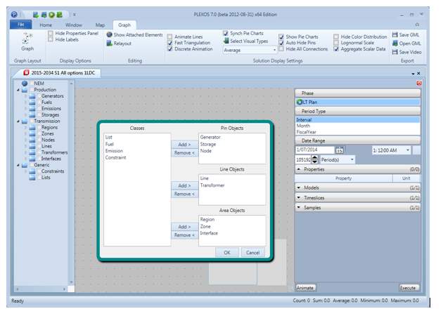
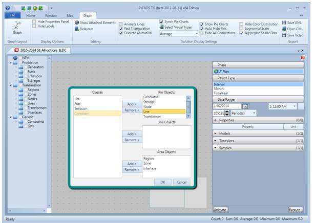
Clicking Select Visual Types opens the above dialog. There is some filtering for line and area objects, user can select line objects only from Lines, Transformers, Waterways, Gas Pipelines and Water Pipelines as well as area objects from Regions, Zones, Interfaces, Lists, Contingencies, Gas Zone and Water Zone.
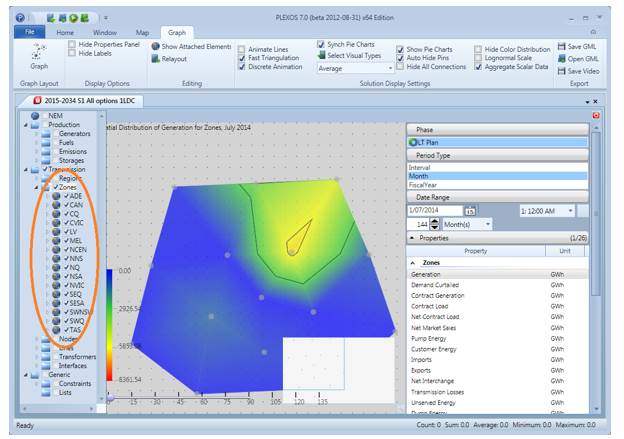
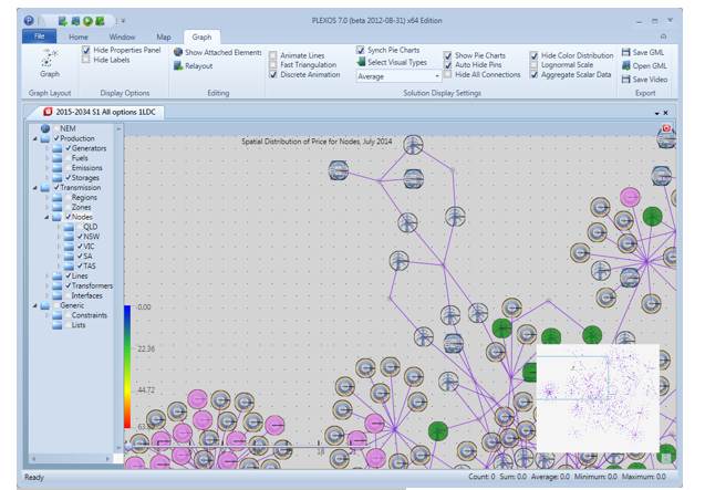
Zones are selected as pin objects, notice the distribution of generation among the zones.
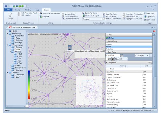
Example: Select generators, storages, nodes, transformers and lines as pin objects.
Generators, storages, nodes, transformers and lines are visualized as pin objects.
Auto Hide Pins icons is on, icons are only visible when mouse hovers over them.
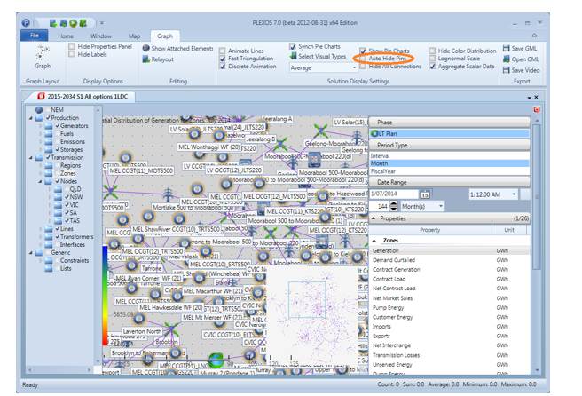
Auto Hide Pins is off, all icons are visible.
Auto Hide Pins is off, Hide Labels and Hid Properties Panel are on.
Lower right corner group's visibility depends on the Search Mode toggle button (looking glass icon) in the very lower right corner of Graph window, works the same way as the search operates in the rest of the GUI.
2.5. Graph Objects
 Line Legend:
- Line: Green
- Transformer: Light Green
- Waterway: Blue
- Gas Pipeline: Cadet Blue
- Water Pipeline: Deep Sky Blue
- Membership: Violet
- Inherited Membership: Magenta
2.6. Manual Positioning
User can arrange pins manually by dragging them to desired positions or use automatic layout option (force-driven layout algorithms are used). Automatic layout works with enabled (in the filters tree) objects.
In order to move any pin object manually, left-press on the pin and drag it to the desired location. Pin selection is done by clicking on a pins icon. Multi-selection is done by holding the Control-key and left-clicking pin objects. Another option for multi pins selection is to draw a rectangle with the left mouse button.
Zoom
Zoom can be adjusted by scrolling the mouse wheel. During a zoom, the point under the mouse remains at the same location and zooming is centred about that point. For the sake of performance, zooming does not update coloured polygons and animation info, undoing the zoom will show areas not covered with colours, and also can zoom during animation without stopping it; in order to update the view, left-click the graph area. Zoom option is only available for Solution viewer.
Full zoom in.
Full zoom out.
User can turn off pie charts to make picture of distribution less crowded.
Or remove coloured surface and view pie charts.
2.7. Execution
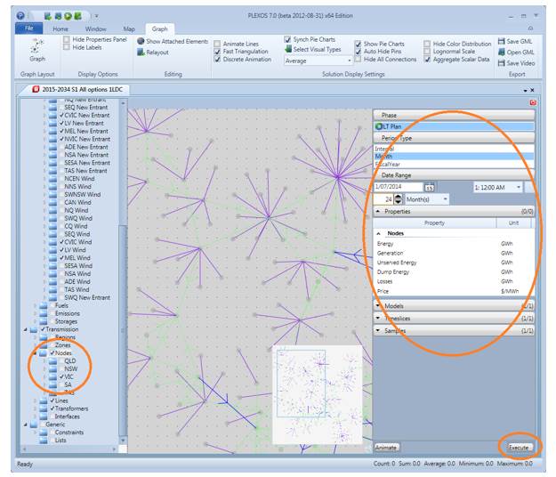
Data retrieving for visualization is organized in a similar way to charts and map visualization. However it is important to put all the objects required to visualize into view before selecting the property to query. After that, select the property to query and click Execute.
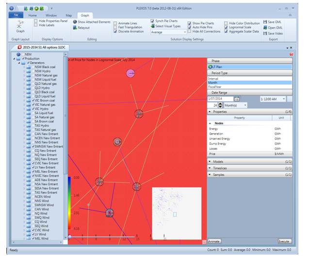
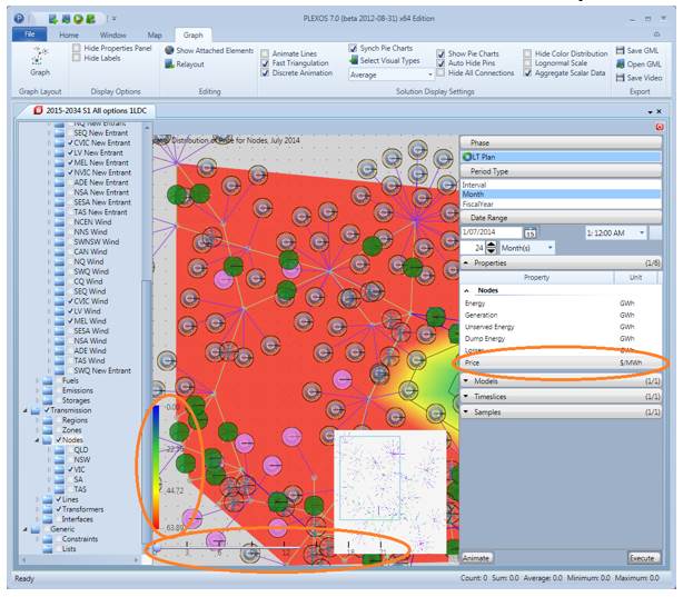
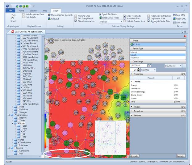
Example: We wish to visualize monthly price for nodes in all available regions for 24 months in LT Plan phase.
Once the property is selected and the query is set, execute the query by clicking Execute in the lower right part of the property selection After the price data has loaded, the selected area is coloured according to the price distribution. The colour - corresponds to a value scale and is shown in the lower left part of the map as a gradient band with several value levels. These value levels are also shown as level lines on the map.
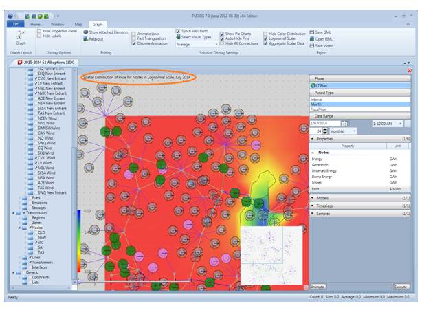
In order to get a picture with more local values (values in nodes affect only neighbouring areas) and smoother value transitions (due to usage of fine regular grid), Fast Triangulation can be turned off.
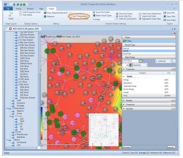
For some properties (like Generation) it makes sense to display spatial distribution with different types of values aggregation. On the picture above there is a generation distribution, when nodes are aggregated (with zoom out) - their Average generation value is used.
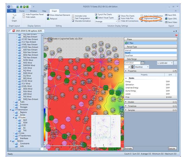
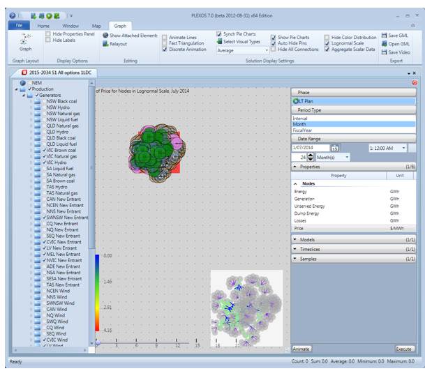
Generation distribution, when their combined generation value is used but in LogNormal scale After Aggregation or Scale mode is changed, press Execute to apply the change. When the selected timeline has more than one timestamp, there is a timeline slider near the left bottom of the map. An animation of distribution changes over the selected period of time can be run using this slider.
The position of the slider indicates the moment of time currently captured and displayed in the animation. It can be used to select a timestamp for a demonstration purposes, dragging the thumb to the desired position will display values at a desired point in time. The timestamp is incorporated into the title at the top of the map.
To start animation press Animate or Resume. Animation can also be saved as an .avi video file. Select Save Video from the Export area and select the location to save the file.
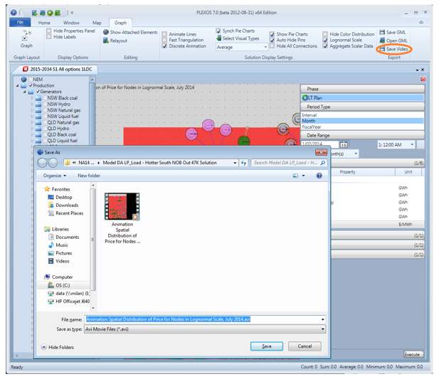
Alternatively, to save the graph itself in .gml format, select Save GML.
3. Hydro Viewer
This chapter introduces graph style visualization functions of PLEXOS GUI for hydro subsystem.
Hydro viewer is a visual layout window which arranges hydro system in such a way, that water flows go from top of the view down to bottom, so that head storage is always placed higher that it's generator and tail storage is always lower, and also storage from is always over storage to for the same waterway. Hydro window can be opened from right-click menu on a collection of storages or waterways in a filters tree of any visual layout.
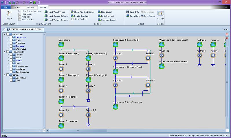
Hydro layout
Items have a context menu, which allows opening property page for an item, show that item on original layout and highlight items connections on Hydro layout.
