Hydro Generator Efficiency and Head Effects
Contents
1. Efficiency
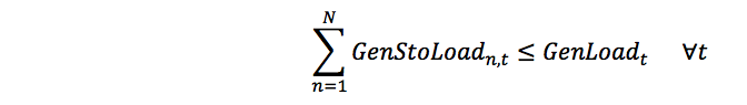
Hydro generator efficiency varies as a function of flow rate using Efficiency Incr in multiple bands with Load Point, usually in combination with the "intercept" term Efficiency Base. An example is shown in Figure 1 (in metric units). In the Level and Volume models, hydro generator efficiency is expressed in electrical energy per unit of water flow through the turbine (cubic metre per second in metric or acre-feet per hour in Imperial US). Examples are shown in Table 1 and Table 2.
The simulator develops a piecewise-linear approximation to this efficiency function, and this is illustrated in Figure 1 (showing flow rates) and Figure 2 (showing volumes of water through the turbine per hour).
NOTE: The number of piecewise linear tranches used is controlled by the Generator Max Heat Rate Tranches property, which defaults to 10. If you provide more than this number of input bands then your input curve is used 'verbatim'. Thus if you wish to input less than 10 bands and want those used by the simulator then set Max Heat Rate Tranches = 1 and input your bands as you want them.
Table 1:Hydro efficiency curve (metric)
| Property | Value | Units | Band |
|---|---|---|---|
| Units | 1 | - | - |
| Max Capacity | 60 | MW | - |
| Load Point | 20 | MW | 1 |
| Load Point | 40 | MW | 2 |
| Load Point | 60 | MW | 3 |
| Efficiency Base | 58 | cumec | - |
| Efficiency Incr | 0.5 | MW/cumec | 1 |
| Efficiency Incr | 0.48 | MW/cumec | 2 |
| Efficiency Incr | 0.42 | MW/cumec | 3 |
Table 2: Hydro efficiency curve (imperial US)
| Property | Value | Units | Band |
|---|---|---|---|
| Efficiency Base | 169 | AF | 1 |
| Efficiency Incr | 171 | kWh/AF | 1 |
| Efficiency Incr | 164 | kWh/AF | 2 |
| Efficiency Incr | 144 | kWh/AF | 3 |
 Figure 1: Generator efficiency - flow rate and piecewise linear incremental efficiency (metric units)
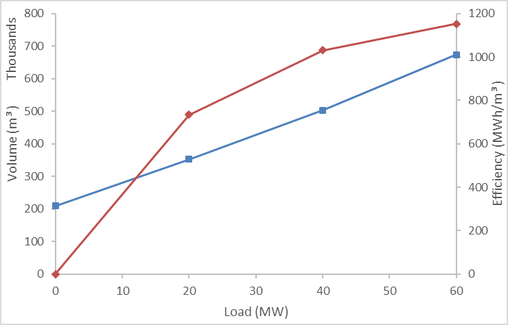 Figure 2: Generator efficiency - water volume and piecewise linear incremental efficiency (metric units)
2. Head Effects
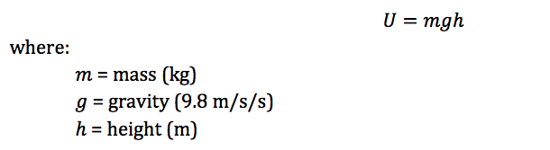
The amount of power produced by a hydro generator is a function of the 'head', which is the difference in height between the head pond and tail pond water levels. The 'head effect' on production efficiency is a function of the gravitational potential energy (U) given by:
Hydro storage is often expressed in volumes of water (cubic metres or acre-feet) rather than height of the storage. Since the shape of the storage is known it is easy to calculate how the potential energy changes as a function of volume. In this case we will follow the example of a trapezoidal storage as shown in Figure 3 with the following parameters:
Table 3: Trapezoidal storage parameters
| Metric | Imperial US |
|---|---|
| High Ref Level = 95 m | High Ref Level = 311.68ft |
| High Ref Area = 342, 530 m^2 | High Ref Area = 3, 686, 967 ft^2 |
| Low Ref Level = 85 m | Low Ref Level = 278.87 ft |
| Low Ref Area = 274, 214 m^2 | Low Ref Area = 2, 951, 616 ft^2 |
| Max Level = 100 | Max Level = 328.08 ft |
| Min Level = 80 m | Min Level = 262.47 m |
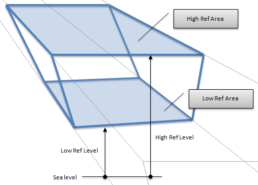
Figure 3: Trapezoidal Storage
The volume of water that can be held in this storage is found by calculating the average of the areas at Max Level and Min Level and multiplying by the height difference. This gives a total volume of 6,167,445 m3 (5000 acre-feet). If we plot the storage volume against the potential energy relative to full volume. The function is quadratic though very close to linear over the range of volumes. We can assume that the generator efficiency is similarly related to the volume.
To define this relationship we divide the storage volume into a series of bands, and enter the efficiency in each band using properties on the Generator Head Storage memberships.
The Generator setting Head Effects Method controls how this is handled in the simulation. According to that setting, the efficiency can be adjusted in a 'backward looking' manner, or directly integrated into the optimization as discussed in the following section.
3. Formulation
When Head Effects Method is set to 'Dynamic' the simulator formulates the head effects directly in the optimization. Here we describe the formulation with an example.
We start with a single Generator object with properties as in Table 4. Note the use of the Scenario "Efficiency Curve" that defines efficiency as a function of flow. In this formulation we allow efficiency be to a function of both flow rate and head.
Table 4: Properties for Hydro Generator
| Property | Value | Units | Band | Scenario |
|---|---|---|---|---|
| Units | 1 | - | 1 | - |
| Load Point | 50 | MW | 1 | Efficiency Curve |
| Load Point | 80 | MW | 2 | Efficiency Curve |
| Load Point | 100 | MW | 3 | Efficiency Curve |
| Efficiency Base | 50 | AF | 1 | - |
| Efficiency Incr | 700 | kWh/AF | 1 | - |
| Efficiency Incr | 937.5 | kWh/AF | 1 | |
| Efficiency Incr | 1250 | kWh/AF | 2 | Efficiency Curve |
| Efficiency Incr | 1125 | kWh/AF | 3 | Efficiency Curve |
We then define the efficiency bands using the properties on the Generator Head Storage membership as in Table 5. Any number of bands may be defined. In this example we define 10 efficiency bands. The Efficiency Scalar values are based on the change in relative potential energy.
Table 5: Efficiency bands for modelling the head effect
| Membership | Property | Value | Value | Units | Band |
|---|---|---|---|---|---|
| Generator (hydro).Head Storage (lake) | Efficiency Point | 95 | % | 1 | |
| Generator (hydro).Head Storage (lake) | Efficiency Point | 85 | % | 2 | |
| Generator (hydro).Head Storage (lake) | Efficiency Point | 75 | % | 3 | |
| Generator (hydro).Head Storage (lake) | Efficiency Point | 65 | % | 4 | |
| Generator (hydro).Head Storage (lake) | Efficiency Point | 55 | % | 5 | |
| Generator (hydro).Head Storage (lake) | Efficiency Point | 45 | % | 6 | |
| Generator (hydro).Head Storage (lake) | Efficiency Point | 35 | % | 7 | |
| Generator (hydro).Head Storage (lake) | Efficiency Point | 25 | % | 8 | |
| Generator (hydro).Head Storage (lake) | Efficiency Point | 15 | % | 9 | |
| Generator (hydro).Head Storage (lake) | Efficiency Point | 5 | % | 10 | |
| Generator (hydro).Head Storage (lake) | Efficiency Scalar | 1 | - | 1 | |
| Generator (hydro).Head Storage (lake) | Efficiency Scalar | 0.982975728 | - | 2 | |
| Generator (hydro).Head Storage (lake) | Efficiency Scalar | 0.965386854 | - | 3 | |
| Generator (hydro).Head Storage (lake) | Efficiency Scalar | 0.947173173 | - | 4 | |
| Generator (hydro).Head Storage (lake) | Efficiency Scalar | 0.928262958 | - | 5 | |
| Generator (hydro).Head Storage (lake) | Efficiency Scalar | 0.908569604 | - | 6 | |
| Generator (hydro).Head Storage (lake) | Efficiency Scalar | 0.887986918 | - | 7 | |
| Generator (hydro).Head Storage (lake) | Efficiency Scalar | 0.866382291 | - | 8 | |
| Generator (hydro).Head Storage (lake) | Efficiency Scalar | 0.843586464 | - | 9 | |
| Generator (hydro).Head Storage (lake) | Efficiency Scalar | 0.819377554 | - | 10 |
The formulation defines binary decisions variables representing operation at times of storage in the given efficiency bands. Specifically we define:
GenStoHeadAbove:
These binary variables are related to the storage volume with the following constraints:
GenStoHeadAbove:

These are the direction analogues of the "Above" and "Below" Constraint objects in the dummy units case.
It also includes a 'choice' constraint that forces the solver to choose to be in one of the efficiency bands:
GenStoHeadChoose:

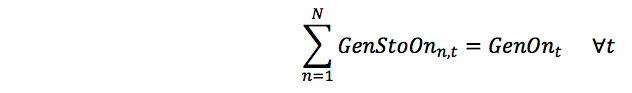
It is not sufficient simply to choose the 'correct' efficiency band, the formulation must now relate generation (GenLoadt) to the efficiency bands. This is done by defining unit commitment (GenStoOnn,t) and generation (GenStoLoadn,t) terms in each efficiency band and additionally (GenStoFann,i,t) for the Fan Approximation of generator efficiency as a function of flow. These terms are linked to generation and the efficiency bands with the following constraints:
GenStoOnDef:
GenStOnUb:

GenStoLoadLb:

Where:
Pmax is the capacity of each generating unit
GenStoLoadTot:
Similar linking equations are defined for the variables. The storage release definition equation now defines release in terms of the original generation and incremental efficiency variables plus modification terms based on the GenStoOnn,t, GenStoLoadn,t(and GenStoFan'_n,i,t') variables:
StoRelDef:
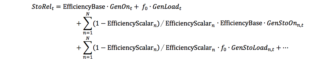
Where:
f0 is the average flow per megawatt hour of generation at full load and reference head level i.e. without modification by Efficiency Scalar.
Note we omit the GenStoFann,i,t terms for clarity.
Figure 4 shows the outcome of modelling with 10 bands for Efficiency Point, Efficiency Scalar and 10 bands for the incremental efficiency function (Fan Approximation) in a full-scale case. The stepwise model of head effects is clearly visible. The spread of efficiencies at each 'step' is a function of the flow through the turbine, with lower flows generally being less efficient.
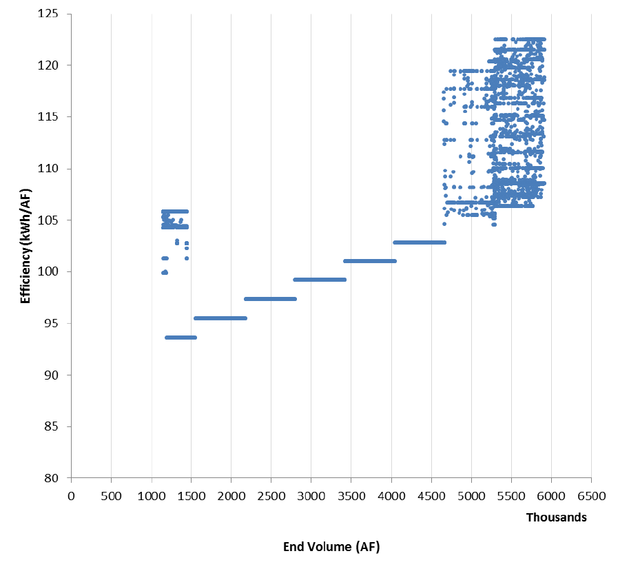
Figure 4: Efficiency versus end volume.