Production Cost Modelling 101
Production Cost Modelling
- Introduction
- Units of Power and Energy
- Power System Dispatch
- Generation Cost
- Transmission
- Market Clearing
- Linear Programming
- Load
- Further Reading
1. Introduction
The purpose of this paper is to provide a first-cut into power system modelling starting with the definition of key terms, and moving into the concepts of power system dispatch, generation cost, load representation, and describing how a system is modelled using mathematical programming.
This paper makes reference to more detailed articles where appropriate.
2. Units of Power and Energy
Firstly some definitions:
- The SI unit of energy is joule (J), equal to one watt-second. it is however a commonly used unit, especially for measuring electric energy.
- The watt-hour (Wh) is a unit of energy; most commonly used on household electricity meters in the form of kilowatt-hour (kWh), which is 1,000 watt-hours.
- One watt-hour is the amount of electrical energy expanded by a one-watt load (e.g. light bulb) drawing power for one hour, and is thus equivalent to 3, 600 joules (1 j/s ->x 1 h x 3600 s/h).
- A kilowatt-hour is 3, 600, 000 joules or 3.6 megajoules.
Utilities tend to use watt-hours to measure energy rather than joules (J), for reasons of convenience and intuition. For example, a light bulb draws power (units of watts) over a certain amount of time, resulting in a net amount of used energy; a watt has units of energy-per-time, and an hour is a convenient unit for measuring time, so when multiplied together they produce a unit of energy called the watt-hour-the amount of power (watts) used for any given number of hours. A light bulb that needs 50 J of energy per second to light up (50 watts) will consume 500 watt-hours of energy (or 3600 × 50 × 10 = 1.8 megajoules) if left switched on for 10 hours.
In the context of a power system model like PLEXOS, we are concerned with the wholesale (and thus bulk) side of electricity production and transmission. Thus the following units are most convenient:
| Element | Unit | Symbol | Conversion |
|---|---|---|---|
| Power (and load) | Megawatts | MW | 1e+6 watts |
| Energy | Megawatt hours | MWh | 1d6 watt-hours |
| Hourly | Volumes of fuel | giga-joules | GJ 1e+9 joules |
| Daily | Volumes of fuel | tera-joules | TJ 1e+12 joules |
| Annual | Volumes of fuel | peta-joules | PJ 1e+15 joules |
The use of joules for energy is a metric convention. Some power systems (e.g. the US) continue to use imperial units. The imperial 'equivalent' to the joule is the British thermal unit (BTU) where:
- 1 BTU = 1055.05585 joules; or
- 1 joule = 0.00094781712 BTU
Hourly volumes of fuel in the imperial system are expressed in mega-BTU (MBTU), which is sometimes written MMBTU. The conversation to metric is thus:
- 1 GJ = 947 817.12 BTU; or
- 1 GJ = 0.9478 MBTU
The following table lists some other important numbers that power system modellers should be familiar with:
| Number | Description | Why it's Useful to Know this Number |
|---|---|---|
| 8760 | Hours in a non-leap year | We often deal with lists of numbers like load forecasts. Knowing this number allows you to quickly check if a set of numbers is a complete year or has data missing. |
| 8784 | Hours in a leap year | As above but for leap year data you should see this many data points |
| 168 | Hours in a week | A week is a common length of time for power system simulation since it is the main cycle of loads. |
| 336 | Half hours in a week | Half hour is a common time period for power market dispatch |
| 17520 | Half-hours in a year | As above but this is for half-hourly data |
| 288 | 5-minute periods in a day | Most markets now dispatch their systems on a 5-minute bases |
| 52 | Whole weeks in a year | Weeks represent natural cycles in power system modelling |
| 3.6 | GJ/MWh for a 100% efficient generator | As a sanity check any heat rate less than this implies an impossibly efficient plant! |
3. Power System Dispatch
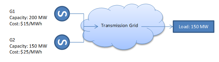
At the most fundamental level, the problem of power system modelling is to determine the least cost dispatch of generating resources to meet a given power demand. By dispatch we mean working out the megawatt production of each plant. An example is shown in Figure 1. Two generators supply power via the transmission grid to a load.
Note:
The following presents a number of scenarios, and the optimal dispatch of the system under each scenario.
Case 1
We require 150 MW of generation to satisfy the load, therefore we despatch* our generators in cost-order from cheapest to most expensive, until the load is met. In this case :
- 150MW from G1 (with 200MW capacity $15/MWh)
- Nothing from G2 (whose cost is higher at $25/MWh)
The total cost to service the 150 MW load is 15 $/MWh × 150 MW = $2250/h NOTE: The ordering of plants by cost is often referred to as the merit-order of generation. Generators that are 'low in the merit-order' are relatively inexpensive, those 'high in the merit order' are expensive, while those that are 'mid-merit' are somewhere in the middle.
Note: The term 'dispatch' is commonly used for the name and the action (rather than the verb 'dispatch').
Case 2
Now, we assume that we require 250MW of generation to satisfy the total load. In this case:
- 200MW from G1 (its maximum capacity)
- 50MW from G2 (the remainder of the load not supplied by G1)
The total cost for 250MW of power would be 15 $/MWh x 200MW + 25 $/MWh x 50 = $4250/h.
Power markets run on marginal pricing thus it is the cost of the marginal (or last) unit of load that sets the energy price. Thus in this case the Price is $25/MWh and thus:
- The cost to load is 25 x 250 = 6250 i.e. what the load pays
- G1 earns Pool Revenue of 25x200 = 5000, incurs Generation Cost of 15 x 200 = 3000, and thus earns a Net Revenue of 5000 - 3000 = 2000.
- G2 earns Pool Revenue of 25 x 50 = 1250, incurs Generation Cost of 25 x 50 = 1250, and thus makes no Net Revenue.
G2 provides the last unit of load and is called the marginal generator.
It is important to note that under a marginal pricing regime the marginal generator is exactly compensated for its incremental cost of the last unit of power generated. Generators further down in the merit order (cheaper) are referred to as infra-marginal and these earn a premium on their generation. Units above the margin are sometimes referred to as extra marginal.
Case 3
In this case, we require the same amount of generation as in Case 2, but loading G1 to its maximum will overload a line in the transmission network. Assuming the maximum load that can be carried from G1 is 180MW then we take:
- 180MW from G1
- 70MW from G2
The total cost for 250MW of power would be 15 $/MWh x 180 MW + 25 $/MWh x 70 = $4450/h
Both G1 and G2 appear marginal in this solution (both could have supplied the 'last' unit of load), but in fact G1 is constrained off i.e. it is generating less than it would economically do: due to the transmission constraint. When a generator is constrained off it cannot be allowed to set the market price, thus G2 is in fact the only marginal generator and the Price =25 (paid by the load) is set by this generator.
And further, the price paid to generators must be consistent with their dispatch level. Thus G1 cannot be paid the market price of 25 because at that price it should have run at maximum capacity. Thus G1 in fact gets paid a price of 15 (equal to its own incremental cost), whereas G2 is paid the market price of 25.
This separation in price is an example of nodal pricing, where the price paid to generators varies according to location. Not all power markets employ nodal pricing; however whatever pricing and settlement system they do adopt the ultimate outcome must closely match nodal pricing for the economic balance to be correct.
Notice in this example the payments that occur:
- The load pays 6250
- G1 and G2 together are paid 4450
- There is a gap or Settlement Surplus of 6250 - 4450 = 1800
This settlement surplus is collected by the market operator and is generally auctioned off to market participants as a way for them to hedge against the price effects of transmission limits.
4. Generation Cost
Power generation has an incremental cost per unit of energy (megawatt hours) based on three key factors:
- The cost of the fuel being consumed.
- The efficiency of generation, which is determined by the technology type.
- The cost of generator maintenance.
4.1. Fuels and Technology
Fuels (in the broadcast sense of the word) fall into three categories
- Fossil: gas, oil, coal
- Nuclear: uranium
- Renewable: hydro, wind, tidal, solar, etc.
The most common thermal generation technologies are:
- Steam: a turbine that uses the heat energy of steam to generate the power for mechanical rotation.
- Gas turbine: an internal-combustion engine in which a turbine is turned by hot gases consisting of compressed air and the products of the fuel's combustion.
Steam plants can run on oil, coal, or gas. Gas turbines require some form of gas: either natural gas or gas produced from coal or other sources. Gas turbine plants come in two main types:
- Combined cycle (CCGT): a gas turbine generator generates electricity and the waste heat is used to make steam to generate additional electricity via a steam turbine; this last step enhances the efficiency of electricity generation.
- Open-cycle (OCGT): here the gas turbine operates independently.
Open-cycle plants are cheaper to construct but are less efficient than combined-cycle plants.
When modelling power systems, and especially when considering expansion of the generation system to meet forecast increases in power demand it is common for the model to consider conventional steam as well as both combined and open-cycle plant as new build options. OCGT plants usually fulfil a 'peaking' role, whereas CCGT, with their greater efficiency operate either as 'baseload' or 'intermediate' plant.
4.2. Efficiency of Generation
Figure 2 illustrates the electricity generation process starting with raw fuel and resulting in electrical energy and waste heat.
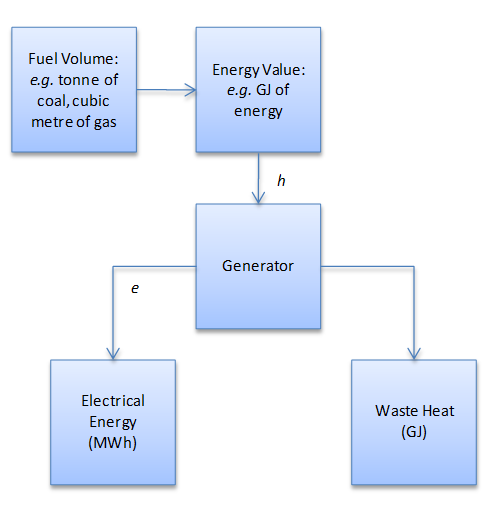 Figure 2: Generation Process
In measuring generator efficiency we refer again to the following definitions:
- 1 watt = 1 joule/sec.
- 1 watt hour = 3600 joules
- 1 MWh = 3.6 GJ
Therefore we can express efficiency as:
Efficiency = 3.6 x (e/h) x 100%
where:
- e = electrical energy output
- h = potential energy input
Additionally we can define:
Heat Rate = (h/e) GJ/MWh
For example:
- h = 1100 GJ
- e = 100 MWh
- Efficiency = (3.6x100) / 1100 = 32.72%
- Heat Rate = 1100/10 = 11 GJ/MWh
4.3. Short-run Marginal Cost
To calculate the unit cost of generation $/MWh (also called the short-run marginal cost or SRMC) we multiply the Heat Rate (GJ/MWh) by the unit of fuels ($/GJ) (Fuel Price):
SRMC = Heat Rate x Fuel Price
alternatively using efficiency:
SRMC = 360/Efficiency × Fuel Price
Note: Heat rate can vary according to generator load level. For SRMC we need the incremental cost of production therefore Heat Rate is strictly-speaking the incremental heat rate i.e. the amount of additional fuel required to make one more unit of power at the current load level.
There are of course other costs to generator operation including;- Operations and maintenance (O&M) costs
- Cost of start up and shut down
- Cost of powering the generator auxiliary loads
- Cost of debt and equity
Some of these costs can be amortised over the amount of generation produced e.g. O&M costs that are a function either of the number of hours of operation and/or the total output over some time period. These so-called Variable O&M costs can be added to the short-run marginal cost of generation thus:
SRMC = Heat Rate x Fuel Price + VO&M Charge
Where the VO&M Charge is equal to the total variable maintenance cost of some period of time (a year for example) divided by the expected total generation in that period. Other costs that cannot be directly attributed to the quantity of generation are referred to as fixed costs and are not counted when computing the short-run marginal cost of generation.
Station auxiliary load, or in-house use, however is partly a function of generation, as well as partly fixed. We distinguish then between the gross (or generator terminal) output of a generator versus the net (or sent-out) generation, where the latter has auxiliary load removed:
Generation (SO) = Generation × (1 - Aux Incr) - Units Generating × Aux Base - Aux Fixed
where:
- Aux Incr is the auxiliary loss for each unit of generation
- Aux Base is the auxiliary load for each unit that is 'on'
- Aux Fixed is the fixed (or permanent) station load independent of generation
Thus the complete short-run marginal cost of generation on a sent-out basis is:
SRMC = (Heat Rate x Fuel Price + VO&M Charge) / (1-Aux Incr)
| Property | Value | Unit |
|---|---|---|
| Heat Rate | 11 | GJ/MWh |
| Fuel Price | 2 | $/GJ |
| VO&M Charge | 3 | $/MWh |
| Aux Incr | 5 | % |
SRMC = (11 x 2+3) / (1-0.05) = 26.32
4.4. Average Versus Marginal Cost
Generators have a range of operation from some minimum stable level up to a maximum capacity, in megawatts. Due to the laws of thermo-dynamics, the incremental cost of generation increases with the amount of load placed on the generator: it costs more to produce each increment of power i.e. the harder you drive an engine the less efficient it gets to produce the next unit of output. However, generation is relatively inefficient at min stable level: the generator takes a certain constant amount of fuel just to run. This constant amount is called the no load cost; therefore the average cost of generation actually falls as you increase output from min stable level. Eventually we reach an optimum point where the average and marginal costs of generation are equal.
An example relationship between the incremental cost and average cost is illustrated in Figure 3. The rising blue line shows the incremental cost of generation (marginal heat rate). Clearly each additional unit of load (output) is costing more to produce in terms of the fuel input, but the red line shows that the average cost of generation (average heat rate) falls as the no-load cost is amortised over more megawatts of output.
If we draw a chart of the total fuel used as a function of generation (Figure 4) we can see that the no-load cost is simply the intercept of this function with the y-axis: though this is an entirely notional point since the generator cannot actually 'run' at zero load.
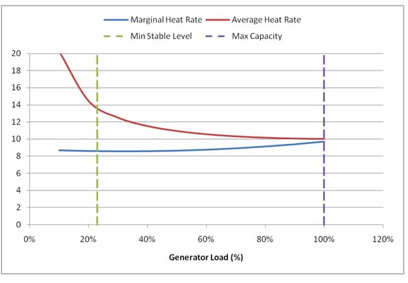 Figure 3: Average versus marginal heat rate
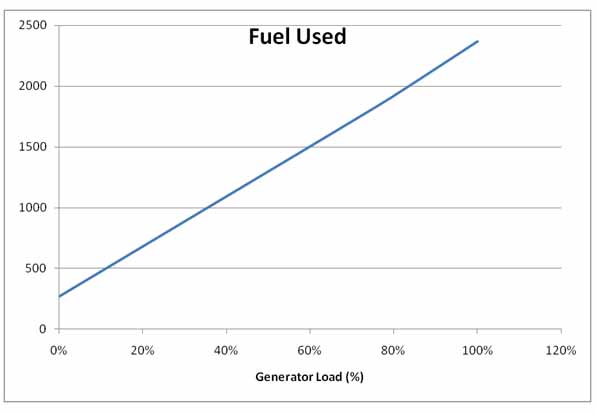 Figure 4: Fuel used as a function of generator load
4.5. Renewables
Renewable generation sources such as hydro, wind, solar, and tidal power, are essentially 'free' (on a marginal basis): with the exception that the generator may require some maintenance costs, which can be assigned to generation. There are however other important limitations such as:
- Hydro generation can be limited by the amount and timing of rainfall and the extent to which water can be stored.
- Solar power only operates during daytime, and varies according to cloud over.
- Wind power is only available when the wind is blowing, and this can coincide with lower power demand times of day.
Because renewables have (near) zero marginal cost they do not set the energy price: which continues to be set by the thermal generator on the margin. If in any period there is no price setting marginal generator, the energy price is zero.
Note that some renewable sources like hydro and pumped storage hydro are able to arbitrage energy between hours of the day, thus reducing the thermal cost in some hours and increasing it in others.
4.6. Hydro Energy
Water stored by a hydro system is potential energy. Hydro systems store this potential energy and make use of it to offset thermal generation costs. The extent to which they can do this is controlled by three factors:
- How much water the system can store: the physical size of the reservoir.
- The timing of rainfall: does it all come at once, or slowly over time.
- The size and efficiency of the hydro turbines: how much that can produce at any one time.
Figure 5 illustrates the typical response of a hydro generator to the energy price. The blue line is the energy price and the green area is the hydro generator output. The plant generates at maximum capacity during high priced periods and at some minimum level otherwise (so-called run-of-river generation). The plant cannot run at full output every period because its total energy is limited.
The operating scheme shown is an example of "peak shaving" i.e. the peak prices are shaved by hydro generation. Simple peak shaving is rarely the optimal solution in a system of any complexity, but solutions should still follow approximately the rule of hydro operating mostly in peak price periods.
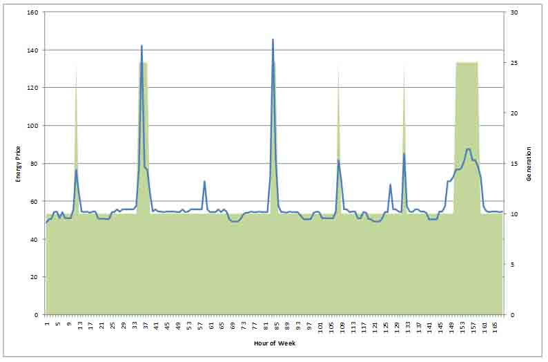 Figure 5: Typical Pattern of Hydro Generation
4.7. Pumped Storage
Hydro plants generate electricity by using gravity to run water through a turbine. Thus water flows from the 'head' storage out the 'tail' of the hydro generator as it operates, and the potential energy of the water is exchanged for electrical energy. A special type of hydro generator called pumped storage has an additional cycle whereby pumps in the station can force water back from the tail pond into the head storage. Of course this requires electricity so the generator swaps from being a generator to load while pumping. For this scheme to be economic the energy price while pumping must be substantially below the price the hydro plant will receive for the generation, thus pumped storage plants show cycles of pumping during low price periods and generating during high priced periods.
Figure 6 shows a typical generation and pumping cycle over a week and the energy prices that drive this cycle. Figure 7 traces the storage level in the head and tail storages respectively for the same cycle. Pumped storages typical run in two cycles, the first across a week, the second within a day, with the highest head water level being at the beginning of the day, and the lowest after the daily peak.
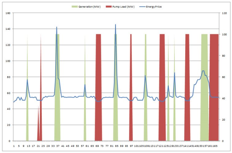 Figure 6: Pumped Storage Cycle
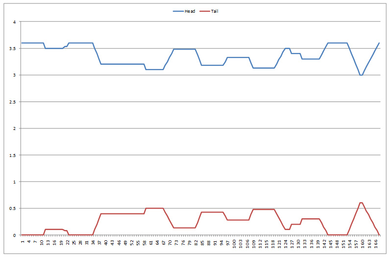 Figure 7: Head and Tail Storage Levels for Pumped Storage
4.8. Technical Constraints
Generators are subject to a number of technical constraints. The following is a glossary of terms commonly used and their meaning:
Min Stable Level Generators are rarely perfectly flexible, but instead have a limited range of operation: either 'off', or 'on' but between some minimum, Min Stable Level (MSL), and maximum, Max Capacity. The minimum is typically around 40% of the maximum. When a generating unit is started it will run as quickly as possible from notional zero output to its MSL. Often this takes less than an hour and so the run-up period is usually ignored when simulating the system. However if the granularity of the simulation is small e.g. 5 minute periods, this run-up can be important and PLEXOS provides inputs (Start Profile) to model this explicitly. Similar comments apply to run-down from MSL to an 'off' state.
Ramp Rate The rate at which a generating unit can change its load level is limited by a number of factors including: the rate that fuel and water for a steam turbine supply can be increased/decreased without taking pressures out of safe ranges; the amount of inertia in the machine itself; manufacturer recommendations; etc. When the ramp rate limit implies that the unit cannot run all the way from MSL to Max Capacity in a single simulation period, then the simulation needs to model the ramp rate as a constraint. Ramp limits are usually expressed as a maximum increase/decrease in megawatts per minute (MW/min).
Start Cost and Time Generators consume some power and fuel when starting. The amount needed is a function of how cold the units are i.e. the time since they were last running. The terms cold, warm, and hot start are used to describe the state of the unit. Generally it is easier and faster to restart a hot unit than a cold one.
Minimum Up and Down Times Thermal generators in particular have minimum running times i.e. a minimum number of hours that, once the unit is 'committed' it must run for, usually expressed in hours and typically in the range of 1-24 hours. Similarly once a unit is shutdown there is sometimes a minimum cooling down period required before the unit can be restarted.
5. Transmission
Loads and generation are rarely situated together: where they are the generation is referred to as 'embedded' generation, or sometimes 'cogeneration'. The majority of generation though is situated away from load centres, and thus the generated electrical power must be transported to the loads. Power systems use alternating current (AC) for transmission: it is preferred to direct current (DC) because it is easier/cheaper to step the voltage down to the safe levels required for domestic consumption: though it suffers higher losses, so some systems use DC links for long distance transmission.
5.1. Laws of Power Flow
Firstly some definitions:
- The term busbar or simply bus is often used in power system modelling to refer to any type of connection point i.e. either a point where two or more lines meet, a transformer between two parts of the network operating at different voltage levels, or a generation connection point. For our purposes, and to avoid confusion, we simply refer to any connection point as a node.
- The term branch is often used to describe a power line. In PLEXOS we use the term line to mean a physical power line (AC or DC).
- We use the term path to refer to a connection in the AC network between two nodes. A path that contains more than one line is called multi-circuit path, and the lines are described as parallel.
- An injection is any electrical generator or load at a point: with generation being a positive injection, and load a negative injection: or withdrawal.
In an ideal world, power could be transmitted from point-to-point directly as required to satisfy load. But the reality is that electrical power flow in an AC network follows a set of rules as described by Kirchhoff:
1. Kirchhoff's Current Law (KCL)The current entering any junction is equal to the current leaving that junction.
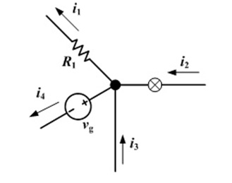 Figure 8: Kirchhoff's Current Law
2. Kirchhoff's Voltage Law (KVL)
The sum of all the voltages around the loop is equal to zero.
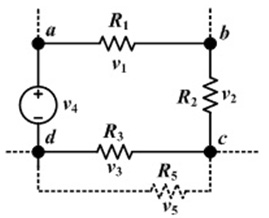 Figure 9: Kirchhoff's Voltage Law
The first law (KCL) simply states that no power can be created or destroyed at any point in the network. In PLEXOS we define the nodal energy balance equations thus:
- Net Injection = Generation-Load
- Net Injection = Exports-Imports
Here, Imports and Exports refer to the flows in and out of the node on the AC network. Net Injection then is the net export of power from the node into the AC network.
The second law (KVL) is more complicated. What it implies is that, in a network with loops (as opposed to a radial network, which has no loops), power will flow around a loop even if the shortest path from generator to load is along one side or other of the loop.
The extent to which power flows on the AC lines in a loop is a function of their impedance. Impedance is a measure of the overall opposition of a circuit to current, in other words: how much the circuit impedes the flow of current. It is like resistance, but it also takes into account the effects of capacitance and inductance. Impedance is measured in ohms, symbol ω. Impedance is more complex than resistance because the effects of capacitance and inductance vary with the frequency of the current passing through the circuit and this means impedance varies with frequency! The effect of resistance is constant regardless of frequency.
Thus it is the combination of injections/withdrawals at the nodes, and line impedances, combined with Kirchhoff's Laws that defines the exact flows around the network.
5.2. Power Flow Example
Consider the 3-bus network in Figure 10. Assume that the impedance of the lines is equal. Now consider the simultaneous injection of 1 megawatt at bus '1' and simultaneous withdrawal at bus '3': KCL dictates that the megawatt injected at bus '1' must flow out of the bus across either path '1->2' or '1->3' or a combination of both to the sum of 1 megawatt. Similarly KCL dictates that the withdrawal at bus 3 is met by flows coming in to the bus on paths '1->3' and '2->3' in some combination.
Figure 10: 3-Bus Example Power FlowsKVL decides exactly what combination of flows occur on paths '1->3', and '1->2'. In this case 2/3 megawatts flows along '1->3' and 1/3 along '1->2', '2->3'. It is easy to see why this would be the case if the lines are of equal impedance, since the direct path '1->3' offers half the impedance of the longer path '1->2', '2->3'.
Note that the power flow laws themselves do not impose any cost on the system, but they do imply a certain set of flows for any given combination of loads and generation, and this affects:
- The real power losses in the network
- The incidence of transmission constraints in the network
For example, referring to Figure 8, some power flows on the path '2->3' even though there is no load or generation at node '2'. This means that a transmission limit could be reached on path '2->3' in the process of sending power between nodes '1' and '3'. Thus modelling these power flow laws is important when simulating a power system.
5.3. Shift Factors
Although the KVL appears complex it can in fact be distilled down to a simple set of factors called shift factors, or alternatively power transfer distribution factors (PTDF). The PTDF are constant for any given network topology (combination of nodes and lines in service). Thus the PTDF can be precomputed and used to calculate the flows in the AC network for any set of injections (generation and load pattern).
A PTDF defines the amount of flow that will occur on a path in the network for a one megawatt increment in the injection at a given node and withdrawal at some arbitrary node. Thus there is one PTDF value for each node and path in the network ([PTDF]_(i,j) where i is the node and j is the path).
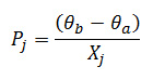
To compute all the PTDF for a network we first form the Y-bus matrix of network impedances:
where:
- X(i,j) is the Reactance of the path between nodes i and j: with zero meaning there is no path between those points.
- The inverse of Reactance is usually referred to as Susceptance and given the symbol 'B':
B(i,j) = 1 / (X(i,j) - When there is no path between two points the reactance and susceptance are zero.
Given Y-bus we now solve the set of linear equations:
Yθ = x
where:
- θ is the vector of phase angles at the nodes in radians (the unknowns)
- x is a vector of injections at the nodes
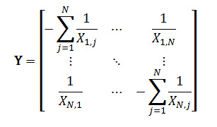
Consider the 3-node example in Figure 8, with the following input for the lines:
| Name | Property | Value | Unit |
|---|---|---|---|
| 1->2 | Reactance | 0.02 | p.u. |
| 2->3 | Reactance | 0.02 | p.u. |
| 1->3 | Reactance | 0.02 | p.u. |
Note the use of the unit 'p.u.' which means "per unit". This convention is used rather than entering ohmic values. Per unit values translate directly into power flows: but because these values are usually very small they are entered using a base of 100 (so called 100 MVA Base). For example a value of 0.02 on a 100 MVA base is actually 0.0002.
Using the above definition, where all the X values are 0.0002, the Y-bus for the system is: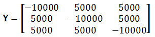
Next we choose a reference point (or slack bus) arbitrarily: let's assume its node '3'. We then eliminate this slack bus from the system (otherwise our system of equations would be over-defined):
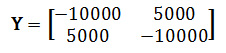
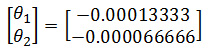
Taking each node in turn: we now solve the set of linear equations (node '1'):
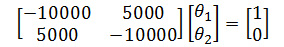
which has the solution:
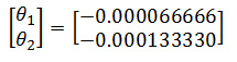
and (node '2'):
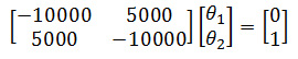
which has the solution:
To compute the PTDF we need to evaluate the flow on each line in the system implied by these phase angle vectors. The flow on a path j flowing between nodes a and b is related to the angles at those buses according to the formula:
For example, the flow on path '1->2' for an injection at node '1' and simultaneous withdrawal at node '3' is:
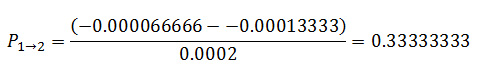
Note that the 'flow' can be negative or positive, where a negative value simply means the flow is in the counter reference direction.
The complete set of PTDF for this case is as follows:
| Injection Point | 0 | 1 | 2 | ||
|---|---|---|---|---|---|
| Path | Bus From | Bus To | 1 | 2 | 3 |
| 1 | 1 | 2 | 0.3333333 | -0.3333333 | 0.0 |
| 2 | 1 | 3 | 0.6666667 | 0.3333333 | 0.0 |
| 3 | 2 | 3 | 0.3333333 | 0.6666667 | 0.0 |
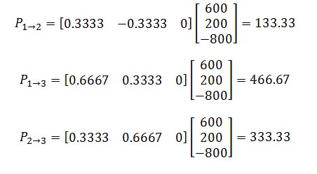
The PTDF can now be used to calculate the flow on any line in the network, given the vector of node injections. For example, if the injections are:
- node '1' generation of 600
- node '2' generation of 200
- node '3' load of 800
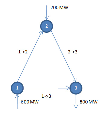 Figure 11: Example Injections in 3-node system
The flows on the three paths are given by:
5.4. DC Lines
AC networks often contain DC lines, especially for bulk transmission over long distances, where DC losses are less than AC. DC lines are subject to the KCL (first law) but not the KVL (second law). Thus in effect a DC line acts simultaneously as a generator and dispatchable load at the nodes it connects where the generation at one end is matched exactly by the load at the other.
Because DC flow is controllable it can be used to 'work around' KVL in the AC network. If we ignore transmission losses, DC lines will only flow when there are constraints in the AC network that can be at least partially relieved by flowing power on the DC. For example, in our 3-node network, with the above flows, imagine now that a DC line of 50 MW capacity is placed between nodes '1' and '3', and set to flow at its full 50 MW:
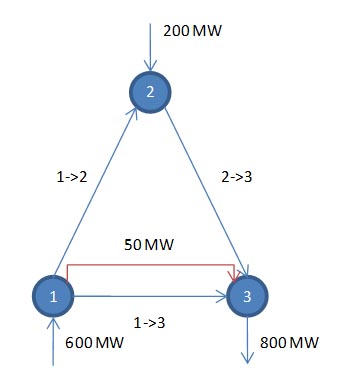 Figure 12: DC Line in 3-node System
The flows in the AC network are computed treating the DC flow as additional injections thus:
This illustrates how a flow on the DC reduces the line loadings in the AC network, and thus can be used to avoid thermal limits (and reduce losses) in the AC network.
5.5. Phase Shifters
Phase shifting transformers (also called FACTS devices) are another mechanism that can be used by the transmission system operator to circumvent KVT therefore reducing the impact of thermal limits caused by loop flow.
From a modelling point of view, a phase shifter can be thought of as a DC line that runs parallel to a line in the AC network. The 'flow limits' on a phase shifter are expressed in terms of the angle difference that they can generate. For example a phase shifter might be able to alter the apparent angle difference between two points by ±5 degrees. We convert this to an equivalent DC line with capacity according to the following formula:
P = ( 2 × π × θ ) / ( 360 × Xj )
where:
- θ is the maximum angle on the phase shifter
- Xj is the reactance of the line
If you place a phase shifter on line '1-2' in the 3-node example, and it had a maximum angle of 5 degrees, it could be modelled as an equivalent DC line with capacity:
P = ( 2 × π × 5 ) / ( 360 × 0.0002 ) = 436.33 MW
5.6. Losses
Up until this point our examples , and equations have assumed that no transmission losses occur in the network. Losses are a quadratic function of power flow:
Lj = Rj x Pj²
5.6. Losses
Up until this point our examples, and equations, have assumed that no transmission losses occur in the network. Losses are a quadratic function of power flow:
Lj = Rj x Pj²
where:
- Rj is the resistance of the line
- Pj is the real power flow on the line
It is beyond the scope of this introduction to describe how losses are treated in a power system model, but PLEXOS can and does model them. Refer to the more detailed articles beginning with Optimal Power Flow - Introduction.
6. Market Clearing
A modern power market acts much like a stock exchange, with generators offering production and loads bidding for supply. The act of clearing the market is much more complicated however because the physical delivery of energy is subject to the limits (and losses) in the transmission network, and potentially many other technical constraints on generation. Further, the market must be cleared every few minutes to ensure continuity of supply to customers, most of whom are not 'bidding' for supply, but whose load is assumed somewhat fixed.
For this reason independent system operators (ISO) operate a centralized power pool through which all trades are made. It is the ISO's task to ensure that the electricity market operates within the physical limits of the transmission system. There are two main types of pool used:
Central Dispatch The ISO manages the physical constraints of both the generation and transmission, and issues instructions to generators for them to start/stop and what generation level to run at.
Self-dispatch Generators make their own on/off decisions and represent their generators' operation using a 'simple' set of Offer Quantity and Offer Price pairs. The ISO only manages the physical constraints of the transmission network, and instructs generators regarding their operating level.
Regardless of the pool type, the ISO typically calculates the dispatch and market pricing solution every few minutes using mathematical programming: linear programming for self-dispatch, and mixed-integer programming for central dispatch: though this is not a hard-and-fast rule.
7. Linear Programming
Linear programming (LP) is a technique for optimization of a linear objective function, subject to linear equality and linear inequality constraints. The real power of LP is its ability to efficiently find the optimal solution to a problem that might have a large number (10's or 100's of thousands of decision variables), where the number of permutations of possible feasible solutions is vast.
Linear programs are problems that can be expressed in canonical form:
- maximize cTx
- subject to Ax ≤ b
x represents the vector of variables (to be determined), while c and b are vectors of (known) coefficients and A is a (known) matrix of coefficients. The expression to be maximized or minimized is called the objective function cTx in this case. The equations Ax ≤ b are the constraints which specify a convex polyhedron over which the objective function is to be optimized. We generally also assume that x requires non-negative values, unless otherwise specified.
7.1. Example
Referring to our simple example in Figure 1 but with the second case where the load is 250 MW: this problem of finding the optimal dispatch could be expressed as the following Linear Program:
minimize 15x1 + 25x2
subject to
- x1 + x2 = 250
- 0 ≤ x1 ≤ 200
- 0 ≤ x2 ≤ 150
Strictly (for canonical form) the equality constraint x1 + x2 = 250 should be written as the pair of inequalities and the objective should be rephrased as maximization thus:
maximize 15x1 + 25x2
subject to
- -x1 - x2 ≤ -250
- x1 + x2 ≤ 250
- 0 ≤ x1 ≤ 200
- 0 ≤ x2 ≤ 150
This linear program involves:
- Two 'decisions variables' ("x1" and "x2") representing the load met by the generators "G1" and "G2" respectively.
- A linear objective function whose value is to be maximized.
- A constraint that ensures that the total generation exactly meets the load.
- Bounds that represent the physical limits of the generators.
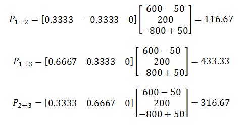
Because it is a two-dimensional problem it can be represented graphically as in Figure 13. Here the constraints are shown in blue with arrows indicating the direction of the inequalities. The so-called feasible region lies along the line x1 + x2 = 250. The optimal solution is found by moving the objective function (in red) upwards until it finds the highest point in the feasible region, as shown in Figure 14. At the optimal solution x1 = 200, x2 = 50 and the objective function value is 4250.
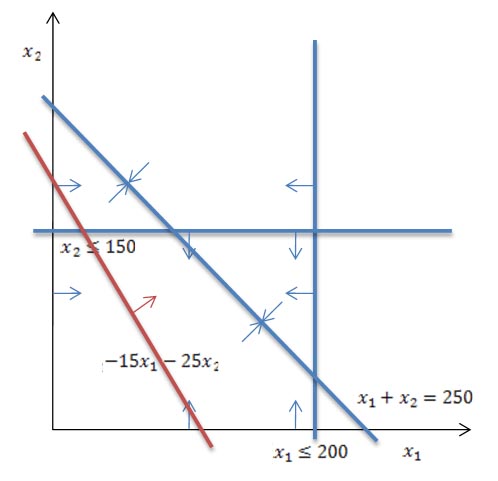 Figure 13: Linear Program
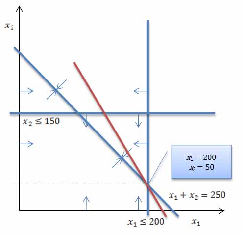 Figure 14: Optimal Solution
7.2. Duality
Every linear programming problem, referred to as a primal problem, can be converted into a dual problem, which provides an upper bound to the optimal value of the primal problem. The dual of a dual linear program is the original primal linear program. For our standard form above the dual is:
- Minimize bTy
- Subject to ATy≥c, y≥0
Relating this to our power system problem:
- The primal problem deals with physical quantities (generation and load). With all inputs available in limited quantities, and assuming the unit prices of all outputs is known, what quantities of outputs to produce so as to minimize total generation cost?
- The dual problem deals with economic values. With floor guarantees on the power price, and assuming the available quantity of all inputs is known, what power price to set so as to maximize the benefit of consumption?
Our example above has the dual:
minimize 250y1 + 200y2 + 150y3
subject to
- y1 + y2 ≥ -15
- y1 + y3 ≥ -25
- y1 free
- y2 ≥ 0
- y3 ≥ 0
The optimal solution is y1=-25, y2=10, y3=0 with objective function value -4250. It is part of duality theory that, at the optimal solution, the primal and dual problems have the same objective function value.
Thus the solution to the dual problem tells us the market price for energy. In our example above that price is $25.00 (when the primal problem is rephrased as a minimization and the dual a maximization). This price is exactly the optimal value of the dual variable associated with the primal constraint that forces generation and load to match.
Note that when a dual variable is zero, the corresponding primal constraint is slack, and vice versa, when a constraint is binding in the primal problem the corresponding dual variable value is non-zero: this is the Complementary Slackness Theorem.
Dual variable values are often called shadow prices (where they apply to constraints in the primal) or reduced costs (where they refer to primal variable bounds).
7.3. Solution Algorithms
There are two solution methods in common use for LP:
Simplex Method Solves the problem by traversing the edges of the feasible region until it finds a point where no further moves can improve the objective function
Interior Point Sometimes called Barrier Method after one variation of the method, it searches through the centre of the feasible region until it reaches the optimal solution.
Interior point is usually supplemented with simplex so that the final reported solution lies at a corner of the feasible region. Such a corner point is referred to as a basis and the associated solution a basic solution. Basic solutions are important because they exploit the duality of Linear Programming.
It is often easier to solve the dual of a problem, and commercial LP solvers will often formulate and solve the dual behind the scenes. Further, solvers might switch at times between performing iterations on the primal and dual problems. Simplex iterations on the primal problem are called primal simplex, and on the dual they are called dual simplex. The revised simplex algorithm switches automatically between these two as it solves according to some rules.
In general, interior point algorithms are fastest on large-scale LP i.e. problems with more than about 250,000 non-zero coefficients in the A matrix. Modern simplex algorithms are generally faster on smaller problems.
Models like PLEXOS do not simply solve one LP but solve a series of them e.g. one for each day or week modelled, and within each of these times steps there can be multiple problems each with small differences like the addition of transmission constraints. When an LP has been solved, and then is resolved with modifications it is often possible to start the LP solution algorithm from the last optimal solution. When this is done it is called either a warm start or hot start: a hot start occurs when only minor modifications have been made e.g. changing an objective function value or right-hand side value, whereas a warm start covers all modifications including adding or deleting entire constraints. Warm or hot starts are always performed using the simplex method and hence if the interior point method is run it is always supplemented with simplex so that warm/hot starts can be done.
7.4. Integer Programming
In a central dispatch model, the ISO makes the on/off ('commitment') decisions for generators as well as deciding the amount of load they will serve. As described earlier, generators have a limited range of operation: either 'off', or 'on' but between some Min Stable Level and Max Capacity. In contrast, our LP above, assumes that generation levels (the decision variables) are continuous so that a generator could operate anywhere between zero and its maximum. To model the discontinuity implied by a minimum stable level we must introduce integer variables into our problem formulation. Integer variables can take values such as 0, 1, 2, ... but not values in between. With integer variables allowed in our formulation we can model the minimum stable level restriction. For example, let's assume that our system has a generating station with three identical generating units each with capacity of 100 MW and minimum stable level of 40 MW, and that the total load is 150 MW. The ISO must decide how many units will be 'on' and at what load level they operate. This can be expressed as the following mixed-integer program (MIP):
minimize 15x1 subject to
- x1 = 150
- x1 ≤ 100x2
- x1 ≥ 40x2
- x1 ≥ 0
- 0 ≤ x2 ≤ 3
- x2 integer
Here x1 is the load met by the generating station in total, and x2 is the number of units turned 'on'. The constraint x1 ≤ 100x2 sets the maximum load that can be met according to how many units are on. The constraint x1 ≥ 40x2 enforces the minimum stable level.
This problem is still two-dimensional and thus can be shown graphically as in Figure 15.
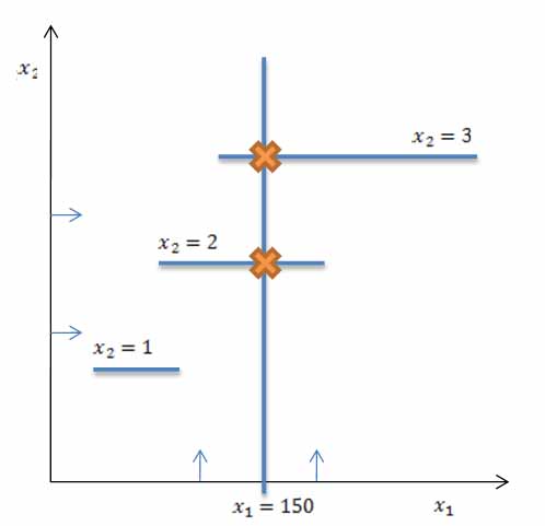 Figure 15: Mixed Integer Program
For each value of the integer variable x2 there is a feasible range for the continuous variable x1. In this simplified example, when the constraint x1 = 150 is considered there are in fact only two feasible points (marked with crosses in Figure 15). The optimal solution is thus either x1 = 150, x2 = 2 or x1 = 150, x2 = 3. In reality (and with more modelling detail) one of these solutions would be preferred (usually the one with less generating units loaded to a higher level).
The important point about mixed-integer programming is that, given a choice of the integer variables, the problem of finding the optimal values for the continuous variables is a linear program. For example, if we set x2 = 3, the mixed-integer program collapses to the LP:
minimize 15x1
subject to
- x1 = 150
- 120 ≤ x1 ≤ 300
Solution methods for MIP explore the space of the integer variables and at each selection solve the corresponding LP. They employ branching and cutting methods so that the number of combinations of integer variables evaluated is much less than a complete enumeration. MIP codes make heavy use of the simplex method to hot start when moving from one combination of integers to another.
Once an optimal integer solution has been found, the corresponding LP (with integers frozen at their optimal values) provides a complete LP solution including the dual information.
8. Load
8.1. Unversed Energy and Dump Energy
In our simple examples above we assume that load is fixed and that consumers will pay any price to meet their load. However the ISO will set a maximum price above which loads would prefer to be 'switched off' than consume energy. This notional price is called the Value of Lost Load (VoLL for short). Likewise our examples assume that generators are flexible and can meet the dispatch instructions of the ISO. Again, there may be cases where the generators in the system cannot reduce output fast enough to meet a drop in load, and thus the ISO may have to set a notional 'dump energy' price below which generators would prefer to be switched off than to operate.
These under and over generation allowances are called Unserved Energy and Dump Energy and act in the market clearing LP like notional generators and loads.
Thus the market-clearing formulation written in words is:
- GenerationCost
- + VoLL x UnservedEnergy
- + PriceofDumpEnergy x DumpEnergy
- Generation - DumpEnergy = Load - UnservedEnergy
- Generation within technical constraints
- Transmission within limits
Thus if generation capacity (or other technical or transmission constraints) imply that the load cannot be met in its entirety, unserved energy will make up the difference, and the market price will be VoLL (generally a very high number like $10,000 per megawatt hour). Likewise, if generation is forced higher than the load, dump energy compensates, and the market price is set to the Price of Dump Energy (generally a number like -1,000$/MWh).
Note that allowing for unserved energy and dump energy in our simulation is necessary to ensure the corresponding mathematical program is feasible, but it is also computationally expensive, for reasons that are beyond the scope of this article.
8.2. Problem Scale
Electrical demand and generation servicing runs in a continuous fashion, with changes in demand being met in real time by changes in generation. For modelling purposes we discretise time into units such as minutes and hours: sometimes called trading periods. For example it is common for power markets to solve the market clearing problem every five minutes with load and generation being metered for settlement at the end of these trading periods.
Especially in the case of central dispatch the trading periods are not completely independent: decisions made in one trading period affect future periods, both physically (in terms of the available generation capacity) and financially (in terms of the cost of starting and stopping units and the choice of generating units online). Thus the market clearing problem is usually formulated as a multi-period optimization. For example, the ISO will dispatch for the current trading period while forecasting the dispatch and pricing outcome for several hours or even days into the future, thus ensuring (assuming accurate forecasting) that the decisions made 'now' are optimal w.r.t. future conditions of load, transmission, and generator availability and costs.
A 'look-ahead' of a few hours to days is adequate for the ISO, but it is in fact not sufficient for general power market simulation. In simulating the system we often want to consider aspects that need to be resolved over longer timeframes than the ISO would consider. These include constraints and financial considerations that are managed by generators through their offers to the power pool but are not considered in the actual market clearing model, such as:
- hydro energy limits
- fuel contract constraints (take-or-pay and maximum availability)
- generator emission limits
- strategic generator behaviour: which is often set over annual periods
When modelling a power system, sometimes we wish to 'simply' emulate the market clearing mechanism right down to modelling every trading period, most times however, and not least for the sake of computation, we use less granularity e.g. modelling using hourly trading periods instead.
Even with this level of simplification however, the problem of simulating a power system over many years and correctly considering these medium term constraints and financial incentives can still prove difficult computationally. There are 8760 hours in a non-leap year. Thus if we wanted to create a market clearing LP that represented an entire year's market operation, so that we could include annual limits on say fuel availability, our LP would be at least 8760 times larger than the one-hour ISO problem. The one hour ISO problem for a system like California can be as large as 100,000 non-zeros (considering 1000's of generators, and 1000's of transmission elements), meaning a year would create a LP with nearly 1 billion non-zeros. At the time of writing no commercial LP code could handle such a large model: the memory required to store such a matrix is at least 156 GB!
8.3. Load Duration Curves
Thus, one of the most important features of a power system simulator is how it deals with these scale issues. PLEXOS solves this problem using a two-stage approach. In the first stage (MT Schedule) load is represented using a technique called load duration curves. In the second stage (ST Schedule) load is represented in its original chronological form but the horizon is split into smaller steps like a day or week: similar to the original ISO problem.
A load duration curve is basically a probability distribution for load. To model a long period of time like a year, we can create a LDC for each day or week or month, that in aggregate is equivalent in energy to the true chronological series of loads. For example, to create a LDC for a week's worth of half-hourly loads like that in Figure 16 we do the following:
- Rank the original values from highest to lowest
- Divide the x-axis into blocks of time
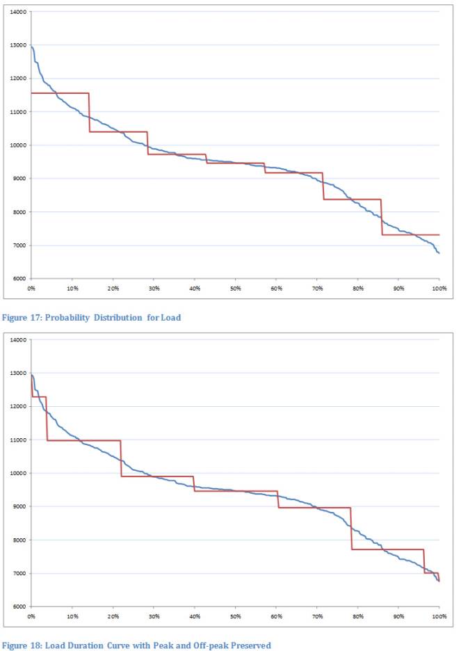
- In each block calculate the average load value as shown in Figure 17
The resulting step function has the same area as the original function, but it misses the peak and off-peak load values, so an alternative is shown in Figure 18 where these values are preserved and the intermediate steps are more spaced out: this is the style of LDC used by PLEXOS.
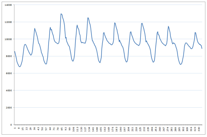 Load Profile for a Week
The LDC is now used as the representation of load and time. Each block of the LDC is associated with it a duration (number of hours). We can formulate our market clearing LP formulation using the number of blocks in the LDC as time periods, and using a weighted-average objective function (where the weights are the number of hours in each LDC block).
To model a year then, PLEXOS creates one LDC for each week of the year, thus with approximately 52 weeks in a year, and if we used seven blocks per week, we have 364 'periods' representing the year (instead of 8760 hours or 17520 half-hours in this case).
Please refer to the MT Schedule documentation for more details on how the solution using LDC is used in the full chronological modelling of ST Schedule.
9. Further Reading
It is recommended that you continue with reading the "Concise User Guide" for an overview of the PLEXOS software and all of its features. More detailed articles are available on individual topics such as transmission and hydro: consult the help for more information.