Region Capacity Expansion Group
| Units: | - |
| Mode: | Input Only |
| Multi-band: | False |
| Default Value: | 0 |
| Validation Rule: | ≥0 |
| Key Property: | No |
| Description: | The capacity expansion group that the region belongs to for LT decomposition. |
Region Capacity Expansion Group is The capacity expansion group that the region belongs to for LT decomposition..
The key motivation behind this feature is the need to model large regional datasets which are generally broken into a number of less coordinated planning regions when it comes to such tasks as transmission planning, capacity markets, and economic forecasts of investment. Generally, these power systems have natural area groups (e.g. sets of Regions) that are virtually transmission-independent, or where the transmission flows between them are reasonably static (e.g. between TSO/ISO). This implies that, once some reasonable estimate of those intertie flows are made, the area groups can be simulated independently.
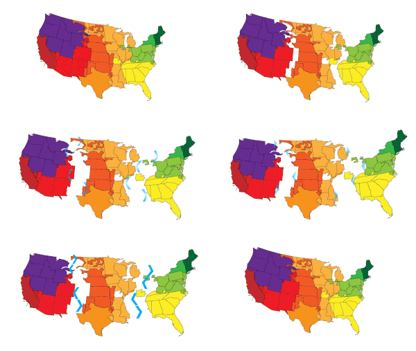
The example data entry provides a decomposition as depicted in the following figure.

Figure 1: Capacity Expansion Decomposition Example
The following points describe the high-level process taken:
Capacity Expansion Group Definition
The user defines the capacity expansion decomposition group/s, by using the Region Capacity Expansion Group property. This essentially instructs the software how the large multi-area models should be split into user-defined decomposition groups, which will run as separate LT simulations.
The group's are to be defined using the Region Capacity Expansion Group property, which is an integer option with a default value of zero. Regions marked as being in the same number group will be simulated together. Thus, by default all are simulated together as they are now, i.e. no decomposition is done. Similarly, if all regions are grouped into the same group then no decomposition is done.
The table below provides an example of how this is defined, along with an explanation of the decomposed outcome:
| Region | Property | Value |
| ISONE | Capacity Expansion Group | 1 |
| NYISO | Capacity Expansion Group | 1 |
| PJM | Capacity Expansion Group | 1 |
| MISO | Capacity Expansion Group | 2 |
| SPP | Capacity Expansion Group | 2 |
| CAISO | Capacity Expansion Group | 3 |
Table 1: Capacity Expansion Decomposition Data Example
This will produce a single dataset with 3 decomposition groups, with the regions "ISONE", "NYISO" and "PJM" in Group 1. Group 2 consists of "MISO" and "SPP", while group 3 has a single region called "CAISO". If there are other regions, which are not defined, then an additional group will be created, which will be numbered as group 0.
Please note, this example is purely to demonstrate how regions can be grouped and is not a suggestion of how regions in the US should be modelled.
Capacity Expansion Group Decomposition
The transmission flows between the groups can be input via Region.Regions Firm Exports. This defines the expected firm export from the Parent Region to the Child Region. Internally those power interchanges will be passed to the smaller individual LT problems as Market objects, with Sales and Purchases defined.
The Market Max Sales and Max Purchases properties are then used to define the intertie ( Line/ Transformer) flows between Decomposition Groups, along with the pricing information.
All this information is processed to produce a single new dataset, with associated settings and datafiles. These data files will all start with the Tilde (~) symbol, indicating that they are temporary files, i.e. they will be deleted at the end of the simulation. This file default behaviour can be changed, so that they persist for your interrogation. This can be disabled via the "Region_DiagnoseDecompositionFiles" hidden parameter.
The set of files created include the following:
- Dataset which is named "~{Dataset name} (Decomposition).xml"
- Data files name in the following format:
- ~{Region name}_Fixed Sales.csv
- ~{Region name}_Fixed Purchases.csv
The temporary outputted datasets will include all models and settings needed to complete the decomposition simulation. The data changes are:
- Added new models based on the decomposition groups defined, e.g. ~CE Group1, along with a scenario with the same name;
- Added Region Units to disable/enabled group regions; these are tagged by the relevant scenario;
- Added Market objects for each region;
- Added Market Max Sales / Min Sales; these are also tagged by the relevant scenario;
- Added Market Max Purchases / Min Purchases; these are also tagged by the relevant scenario;
The CSV files are simple data files, containing the decomposed values from the LT or MT phase.
Solution Gathering
When the smaller LT simulations are completed, the builds and retirements for each Capacity Expansion Groups are written to csv files. Note that this functionality currently only works for the Electric model. The builds and retirements are then fixed in the main problem and the simulation of all phases continues with the fixed builds
See also: