Region Decomposition Group
| Units: | - |
| Mode: | Input Only |
| Multi-band: | False |
| Default Value: | 0 |
| Validation Rule: | ≥0 |
| Key Property: | No |
| Description: | The decomposition group that the region belongs to. |
| Detail: |
The Region Decomposition Group property is the key setting to enable the geographical decomposition functionality.
The key motivation behind this feature is the need to model very large multi-area energy models, that are generally slow to run at the higher resolutions in ST Schedule. Generally, these power systems have natural area groups (e.g. sets of Regions) that are virtually transmission-independent, or where the transmission flows between them are reasonably static (e.g. between TSO/ISO). This implies that, once some reasonable estimate of those intertie flows are made, the area groups can be simulated independently.
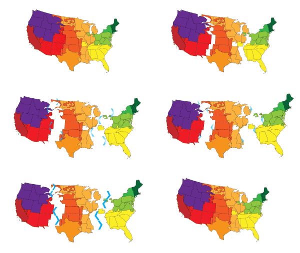
The example data entry provides a decomposition as depicted in the following figure.

Figure 1: Geographical Decomposition Example
The following points describe the high-level process taken:
Group Definition
The user defines the decomposition group/s, by using the Region Decomposition Group property. This essentially instructs the software how the large multi-area models should be split into user-defined decomposition groups, which will run as separate simulations.
The group's are to be defined using the Region Decomposition Group property, which is an integer option with a default value of zero. Regions marked as being in the same number group will be simulated together. Thus, by default all are simulated together as they are now, i.e. no decomposition is done. Similarly, if all regions are grouped into the same group then no decomposition is done.
The table below provides an example of how this is defined, along with an explanation of the decomposed outcome:
| Region | Property | Value |
| ISONE | Decomposition Group | 1 |
| NYISO | Decomposition Group | 1 |
| PJM | Decomposition Group | 1 |
| MISO | Decomposition Group | 2 |
| SPP | Decomposition Group | 2 |
| CAISO | Decomposition Group | 3 |
Table 1: Geographical Decomposition Data Example
This will produce a single dataset with 3 decomposition groups, with the regions "ISONE", "NYISO" and "PJM" in Group 1. Group 2 consists of "MISO" and "SPP", while group 3 has a single region called "CAISO". If there are other regions, which are not defined, then an additional group will be created, which will be numbered as group 0.
Please note, this example is purely to demonstrate how regions can be grouped and is not a suggestion of how regions in the US should be modelled.
Group Decomposition
The transmission flows between the groups are calculated by first running a lower resolution simulation and recording the Line/Transformer flows between the groups, then passing those power interchanges to the high-resolution Decomposition Group runs as Market objects, with Sales and Purchases defined.
The low-resolution run will be either LT or MT, depending which phases are selected. If both phases are selected, then MT is considered to have a "higher resolution", so is utilized for the flow calculations. These flow calculations record the Line/Transformer flows between the decomposition groups defined, along with the regional pricing information. The Market Max Sales and Max Purchases properties are then used to define the intertie ( Line/ Transformer) flows between Decomposition Groups, along with the pricing information.
All this information is processed to produce a single new dataset, with associated settings and datafiles. These data files will all start with the Tilde (~) symbol, indicating that they are temporary files, i.e. they will be deleted at the end of the simulation. This file default behaviour can be changed, so that they persist for your interrogation. This can be disabled via the "Region_DiagnoseDecompositionFiles" hidden parameter.
The set of files created include the following:
- Dataset which is named "~{Dataset name} (Decomposition).xml"
- Data files name in the following format:
- ~{Region name}_Fixed Sales.csv
- ~{Region name}_Fixed Purchases.csv
- ~{Region name}_Price.csv
The temporary outputted datasets will include all models and settings needed to complete the decomposition simulation. The data changes are:
- Added new models based on the decomposition groups defined, e.g. ~Group1, along with a scenario with the same name;
- Added Region Units to disable/enabled group regions; these are tagged by the relevant scenario;
- Added Market objects for each region;
- Added Market Max Sales / Min Sales; these are also tagged by the relevant scenario;
- Added Market Max Purchases / Min Purchases; these are also tagged by the relevant scenario;
The CSV files are simple data files, containing the decomposed values from the LT or MT phase.
Solution Gathering
When the simulations are completed, the individual group solutions will be combined a single database.
This process invokes the stitch functionality and will search for all simulated solutions completed successfully. It will then combine all of these into a solution file, which can be browsed as normal. Should one of the "group simulations" fail, the information will be omitted from the final solution file.
Connect Simulation
Using Connect (version 3.3R01 or higher) to launch a decomposition simulation will result in the decomposition groups being distributed to any of the client machines available. Once completed, the solution information is gathered and a final output solution database is generator.
Please note, that a decomposition simulation will only consume a single license, regardless of the number of decomposition groups being used.