Load Forecasting
Contents
1. Introduction
The Data File class can be used to create load (or other) forecasts for input to a simulation. The load forecasting exercise takes as input:
- A "base" year's profile of demand i.e. period-by-period demands;
- A forecast of total energy (GWh) and maximum demands (MW) over the forecasting horizon; and optionally.
- A forecast of minimum demands (MW) over the forecasting horizon; and optionally.
- A list of holiday periods that must be preserved in mapping the forecast years to the base year.
The base profile must be stored in a PLEXOS format text file e.g. CSV or TXT file. Note that if you use a named format, the names in the files must match the name of the Data File objects they are associated with (which may be different to the names of the objects that eventually use the data as input in the simulation). Likewise, the output forecast will always be created in a text file, see [1].
All these data (input and output) are stored on Data File objects. You should create one Data File object per forecast file you wish to create.
2. Defining the Input Data
2.1. Filename Property
The input property Filename points to the output filename for the load forecasting exercise. This property is the "key" property of the Data File class. When using the Data File to provide data to the simulation it is the Filename property that is used to access the data. There should be only one Filename entry and you cannot use scenarios here (to create multiple different forecast scenarios you must use separate Data File objects).
There are three fields that should be filled out in the Filename entry. Firstly the Filename field should contain the name of the text file that is going to hold the forecast output. Next, the Date From and Date To fields should contain the start and end dates for the forecasting horizon. These should be exact beginning and end points for years and not include time parts. For example to create a forecast for calendar years 2003 to 2013 the Date From should be 1/1/2003 and the Date To should be 12/31/2013.
2.2. Base Profile Property
The Base Profile property points to a text file in the same way as the Filename property, but this is the file that will be used to define the historical (or base) year from which the forecast profiles are generated. You must fill in the Date From field with the first day of the base profile year even if the text file only contains one year's data. Note that neither the forecast nor base years need to be calendar years - fiscal years can be used. The text file used to define the Base Profile property can contain data for more than one year, however only one year's data will be read, starting from the Date From specified date.
2.3. Energy and Maximum Properties
The properties Energy and Maximum together define the load forecast. The Energy property is in units of GWh total demand and each Energy entry must have the Date From field set to indicate the year the energy applies to. The Maximum property likewise applies to the maximum demand. The Maximum can be set multiple times inside a year or with a pattern e.g. to indicate summer and winter maximum demands. There apply some restrictions on the form of the input data for Energy and Maximum properties. The definition of these properties using Condition, Variable, Escalator, Data File or Scenario is not supported. Energy and Maximum properties can only use Date From, Date To, and Timeslice in raw patterns format (not pointing to a Timeslice Object) entries.
2.4. Minimum Property
Minimum is an optional property could be added together with Energy and Maximum to define the load forecast. It should have the same form/pattern of the input data as Maximum. See above.
2.5. Holiday Property
By default the growth algorithm will preserve days of the week when producing the forecast profiles i.e. each Monday will be derived from a related Monday in the base profile. But holiday periods may get moved around unless they are explicitly defined. The Holiday property is used to define a holiday. To define a holiday you must indicate:
- When the holiday appears in the base profile by creating a Holiday property with Date From and Date To inside the base year.
- What day the same holiday appears in each forecast year by creating Holiday properties with the Date From inside each forecast year.
Multiple holidays can be defined using different band numbers e.g. the first holiday in the year can be on band 1, the second on band 2, etc. There is no limit to the number of holiday periods that can be defined. Note though that holidays can be for multiple days but must be contiguous in every year. Thus holidays that get split across a weekend must be split into two holidays.
2.6. Example
In the following example a load forecast is being created from the 2008 calendar year historical demands. The forecast is for 1 year (2009). There are nine holiday periods (defined on nine bands). The holiday is enabled if its value is "Yes". For all holidays in the same band, just the holiday's value of base year counts. Take holidays of band 1 as an example, if the holiday's value at 1/01/2008 is "Yes", then no matter the holiday's value in 2009 is yes or not, all holidays in band 1 are enabled. In contrast, if the holiday's value at 1/01/2008 is "No", then no matter the holiday's value in 2009 is yes or not, all holidays in band 1 are not enabled.
If 1/01/2009 is defined as holiday and its base holiday is enabled and defined as 1/01/2008 (it can be defined as any other day in 2008), just like the case in the following table, in the process of producing load forecasting, the load forecast of 1/01/2009 will be calculated based on the load value of 1/01/2008 even 1/01/2008 is Tuesday and 1/01/2009 is Thursday. Furthermore, if 1/01/2009 is not defined as holiday or its base holiday (1/01/2008) is not enabled, then the date in 2008 which in the same week, same day of the week as 1/01/2009 in 2009 will be picked as based value. For example, 1/01/2009 is the 4th day (Thursday) of the 1st week in the year, in 2008, the 4th day of the 1st week is 3/01/2008. So, the load forecast value of 1/01/2009 will be calculated based on the value of 3/01/2008. If 3/01/2008 happened to be a holiday, then, check the previous week and then next week.
Rare case is for example, the Tuesday of ith week of 2009 should match the Tuesday of ith week of 2008, but that Tuesday in 2008 is holiday and the Tuesday in (i-1)th and (i+1)th week in 2008 is holiday too, then, it will find its match starts from the Tuesday of ith week of 2008 to the Tuesday of the 1st week of 2008. If i happens to be the first week, then find its match starts from the last week of 2008.
| Property | Value | Filename | Units | Band | Date From | Date To |
|---|---|---|---|---|---|---|
| Filename | 0 | Load_LADWP_out.csv | - | 1/01/2009 | 31/12/2009 | |
| Base Profile | 0 | Load_LADWP_base.csv | - | 1 | 1/01/2008 | 1/01/2008 |
| Energy | 53061 | - | - | 1 | 1/01/2009 | 31/12/2009 |
| Maximum | 9493 | - | - | 1 | 1/01/2009 | 31/12/2009 |
| Holiday | Yes | - | Yes/No | 1 | 1/01/2008 | 1/01/2008 |
| Holiday | Yes | - | Yes/No | 1 | 1/01/2009 | - |
| Holiday | Yes | - | Yes/No | 2 | 28/01/2008 | 28/01/2008 |
| Holiday | Yes | - | Yes/No | 2 | 26/01/2008 | - |
| Holiday | Yes | - | Yes/No | 3 | 10/03/2008 | 10/03/2008 |
| Holiday | Yes | - | Yes/No | 3 | 1/01/2008 | 9/03/2008 |
| Holiday | Yes | - | Yes/No | 4 | 21/03/2008 | 21/03/2008 |
| Holiday | Yes | - | Yes/No | 4 | 10/04/2009 | - |
| Holiday | Yes | - | Yes/No | 5 | 24/03/2008 | 24/03/2008 |
| Holiday | Yes | - | Yes/No | 5 | 13/04/2009 | - |
| Holiday | Yes | - | Yes/No | 6 | 25/04/2008 | 25/04/2008 |
| Holiday | Yes | - | Yes/No | 6 | 27/04/2009 | - |
| Holiday | Yes | - | Yes/No | 7 | 9/06/2008 | 9/06/2008 |
| Holiday | Yes | - | Yes/No | 7 | 8/06/2009 | - |
| Holiday | Yes | - | Yes/No | 8 | 25/12/2008 | 25/12/2008 |
| Holiday | Yes | - | Yes/No | 8 | 25/12/2009 | - |
| Holiday | Yes | - | Yes/No | 9 | 26/12/2008 | 26/12/2008 |
| Holiday | Yes | - | Yes/No | 9 | 28/12/2008 | - |
3. Building Forecasts
3.1. Invoking the Build Algorithm
Having created the input data for one or more Data File objects the forecast algorithm is invoked using the Build command (either on the toolbar or on the right-mouse button menu for Data Files). Use the Add/Remove buttons to move the Data Files that wish to build into the right-hand section of the form. You can also choose the format of output file. Note that "Periods in Columns" format is most compact, while "Bands in Columns" is easier to graph directly, e.g. in Excel, if required. Note that you can view any selected Data File from the build window before or after building it.
To invoke the data file build, click the OK button. Firstly the program will check that all required data are correctly defined and will report errors if any data are incorrect. Then the application will show progress of the load growing algorithm. Each year of each file takes a few seconds to construct. Once all selected files are created you will be returned to the Data Files page where you can view the results using the View button.
4. Advanced Usage
The forecast profiles are built using a mathematical model. The forecast energy and maximum (and minimum if defined) are always obeyed. The Data file Method by default is equal to 1 (the default "linear" method) and can be set to 2 (quadratic method). These two growth methods are suitable for most applications, but can have problems if the implied growth rate of the maximum (minimum) and energy are very different. In this case you can instruct the builder to use quadratic method with more specific settings.
In the quadratic method, you could also specify the Relative Growth at Min parameter, which enforces a constraint that ensures that the specified amount of growth (relative to the growth of the energy) is applied to the tail of the load duration curve e.g. if the energy is growing at 4% and the maximum at 15%, you can try a value for this parameter of 50%, which implies the minimum observation will grow by 4% × 0.5 = 2%. In the opposite case in which energy is growing more than the maximum, this parameter should be > 100%. In these cases, the Minimum property should not be defined otherwise the constraints might be conflict.
4.1. Example: Maximum Growing Faster Than Energy
In this example the energy is growing at 6% relative to the base year (2000/01), but the maximum is growing at 15%. Figures 1 and 2 show the time series and load duration curve produced by the linear method compared with the base year. The shape of the series becomes distorted by the very high maximum growth relative to energy and the result is that some of the lower observations actually have negative growth. Switching to the quadratic method can resolve this problem, by setting:
| Membership | Property | Value | Units |
|---|---|---|---|
| Data File (VIC1) | Method | 2 | - |
| Data File (VIC1) | Relative Growth at Min | 10 | % |
The resulting time series and load duration curve is shown in Figures 3 and 4.
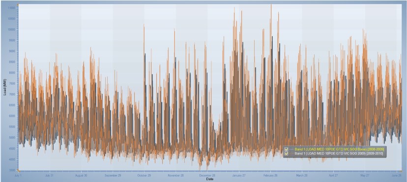 Figure 1a: Time series from the linear method (Annual summary view)
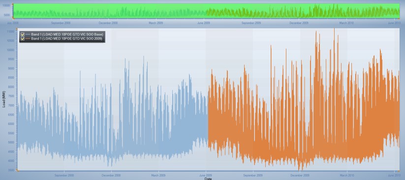 Figure 1b: Time series from the linear method (Series view)
 Figure 2: Load duration curve from the linear method
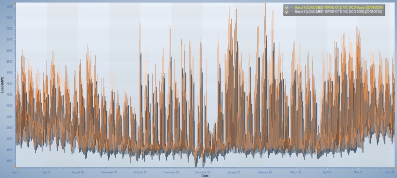 Figure 3a: Profile from the quadratic method (Annual summary view)
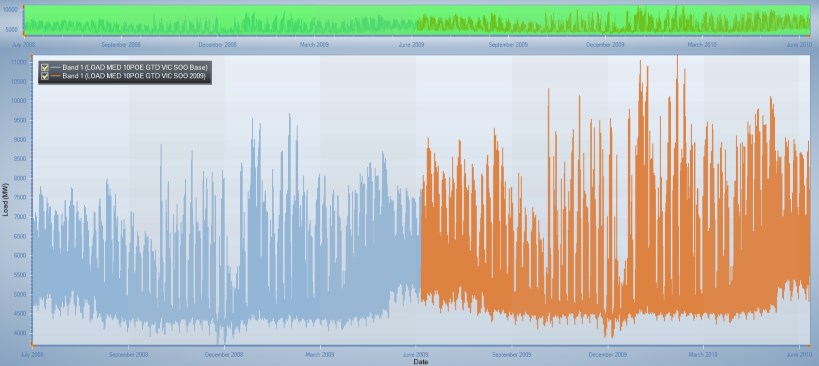 Figure 3b: Profile from the quadratic method (Series view)
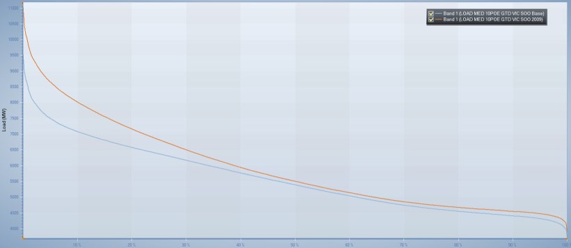 Figure 4: Load duration curve from the quadratic method
4.2. Example: Energy Growing Faster than Maximum
In this example the energy is growing at 28% relative to the base year (2002), but the maximum is growing at only 9%. Figures 5 and 6 show the time series and load duration curve produced by the linear method compared with the base year. The shape of the series becomes distorted by the very high growth produced at the lower end of the load duration curve. The result is an unacceptable change in the load factor of the forecast.
Switching to the quadratic method can resolve this problem, by setting:
| Membership | Property | Value | Units |
|---|---|---|---|
| Data File (VIC1) | Method | 2 | - |
| Data File (VIC1) | Relative Growth at Min | 33 | % |
| Data File (VIC) | Max Shape Distortion | 0.6 | % |
The resulting time series and load duration curve is shown in Figures 7 and 8.
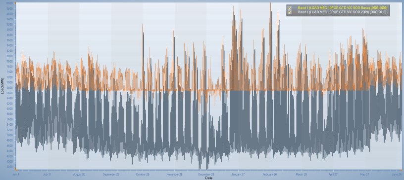 Figure 5a: Profile from the linear method (Annual summary view)
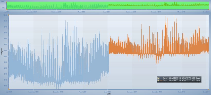 Figure 5b: Profile from the linear method (Series view)
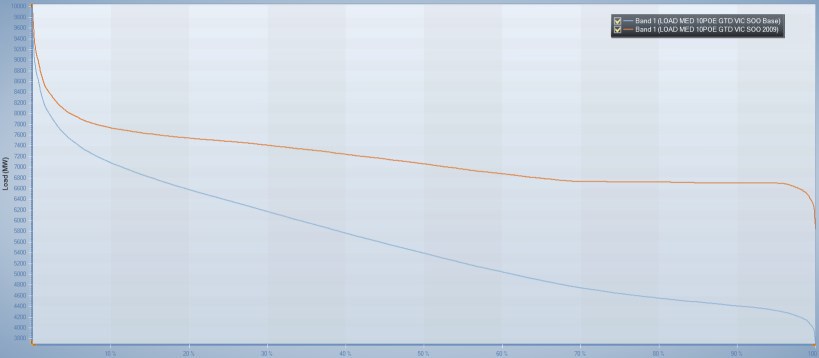 Figure 6: Load duration curve from the linear method
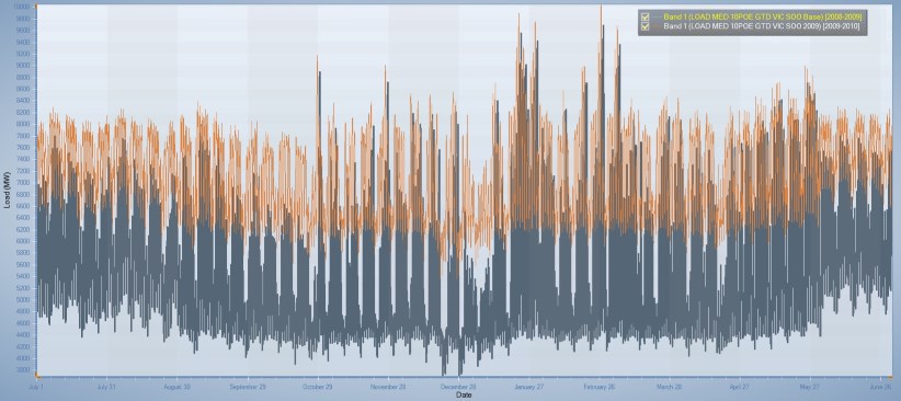 Figure 7a: Profile from the quadratic method (Annual summary view)
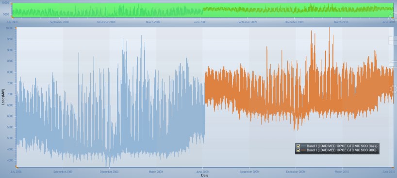 Figure 7b: Profile from the quadratic method (Series view)
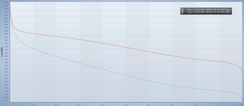 Figure 8: Load duration from the quadratic method