Multi-Objective Modelling
Contents
1. Introduction
Multiple objectives can be defined to analyse the trade off between competing objectives using Lexicographic (or hierarchical) optimization and blended (weighted average) optimization. The multi-objective feature can be defined and implemented through the Objective class, with its main properties being:
| Properties | Description |
|---|---|
| Sense | Sense in which the objective has to be optimized |
| Priority | Priority of the objective when doing hierarchical multi-objective optimization. |
| Weight | Weight of the objective when doing blended multi-objective optimization. |
| Constant | Constant is Objective constant. This does not affect any optimization mathematically. |
There are two types of multi-objective optimization: Lexicographic (or hierarchical) and Blended (or weighted sum/average). The Lexicographic is used when the user knows that there is clear order in which the objective functions are prioritized. System Cost is the default PLEXOS objective and always has the highest priority. Blended is used when the user wants to solve for a trade off between two objectives. Blended is the approach one should prefer in case they want to explore the entire Pareto-Optimal front.
2. Types of Multi-Objective Modelling
2.1. Lexicographic or Hierarchical
A series of optimization problems are solved at each step based on priority as shown in Figure 1.
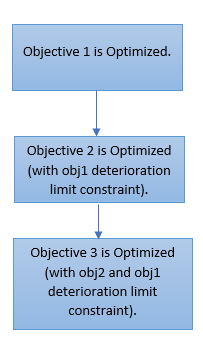 Figure 1: Hierarchical Multi-Objective Modelling
In case two objective functions have the same priority, then for that step blended approach is used to consolidate both the objectives into single objective function.
2. Blended or Weighted Sum
In Blended Approach we consolidate the objective functions into a single objective using weights.
Say there are two objective functions f1 and f2, with weights w1 and w2 respectively. The blended objective is given by:
- w1*f1 + w2*f2
- for n objective functions this extends to: w1*f1 + w2*f2 + ... + wn*fn
3. Pareto-Optimal Front
Blended Approach can be used to generate a Pareto-optimal front in lower dimension objective space. Say we have two functions f1 and f2 with weights w1 and w2 respectively. We can solve a series of multi-objective models where weights w1 and w2 are complementary convex sum of 0 and 1 (w1 + w2 = 1, w1 >=0, w2>=0). By solving a series of models ranging from {(w1,w2)=(0,1}} to {(w1,w2)=(1,0}}, we could get a series of functional value pairs (f1,f2). Plotting the functional values (f1,f2) will generate the Pareto-Optimal front as shown in Fig
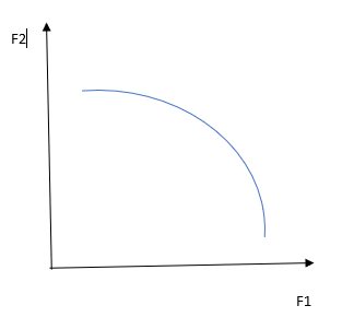 Figure 2: Pareto-Optimal Front
We would recommend that the sense of all objective functions be same in case one is exploring for Pareto-Optimal front. The sense can be reversed for the purpose with a negation if required. Pareto-optimal fronts can be visualized up to 3 - objective functions. This visualization has to happen outside PLEXOS. Pareto-Optimal fronts can be discontinuous and therefore a high resolution of (w1,w2) iteraties is required to get a smooth curve.
4. Multi-Objective Example
Here is an example for setting up a multi-objective optimization problem with the total CO2 emissions as the second objective:

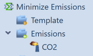
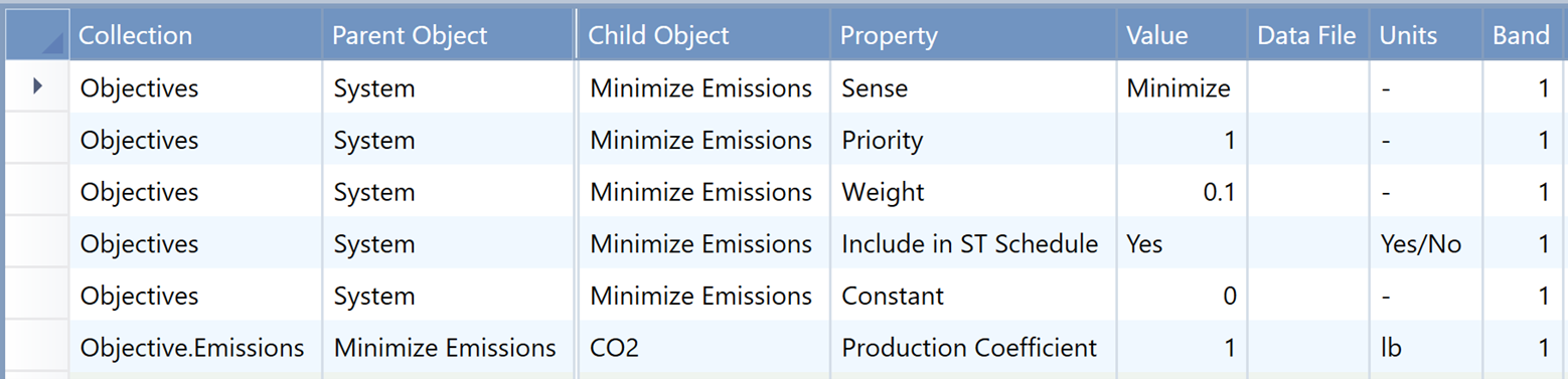
The Minimize Emissions objective has a Priority of 1 and a Weight of 0.1. The only membership with the objective is the CO2 emissions object which has a Production Coefficient of 1, meaning that the objective is to minimize the total CO2 emissions. Note that the Constant property needs to be defined, even if it is zero. The Priority and Weight of the base (total cost) objective are defined on the model itself, and in this case are both set to 1:
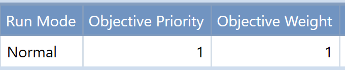
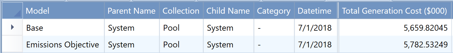
Since the Priority of both objectives are the same, the optimization will use the blended approach so that the final objective used in the optimization is to minimize the total system cost plus 0.1 multiplied by the total emissions. Here is a comparison of the emissions of two simulations run with and without the second objective included:
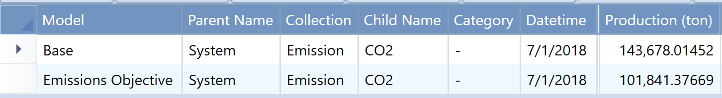
The total emissions decreased significantly with the emissions objective, but the total system cost also went up as expected: