Transmission - Locational Marginal Prices

Contents

1. Introduction
2. Energy Change
3. Congestion Charge
4. Marginal Loss Charge
5. Marginal Loss Factor

1. Introduction

Kirchhoff's Laws require that power imports and exports are balanced at each node of the network and that power flows with respect to KVL. These two rules are in fact implied by the network shift factors. Thus the DC-OPF balances supply and demand only at the system level and not specifically at the node level. The dual solution to the production cost problem above gives no information about the nodal prices. In this section we describe how the nodal prices are calculated from the optimal solution to the production cost problem with DC-OPF.

2. Energy Change

A nodal price represents the cost to the system as a whole of a unit change in load at the bus. In the absence of either constraints or losses all nodal prices will be equal. This uniform price is referred to as the system lambda or network energy charge. No matter where we perturb load in the network, the marginal impact on total system cost would be the same.

As we introduce constraints on the transmission flows (either on individual branches or combinations of flows), the nodal prices diverge. Losses also cause separation of prices across the network. In this case there is no easily recognisable system lambda. But we could compute a system lambda by choosing a combination of load/generation buses to increment/decrement and compute the change in total system cost:

where:

• λ is the system lambda
• δC is the change in total system cost
• δD is the change in load

The choice of load/generation buses is rather arbitrary. However, in the DC-OPF there is a natural choice of buses being the slack bus(es). And further, the formulation of this model naturally provides the corresponding system lambda: it is the shadow price (dual variable) on the supply/demand balance constraint:

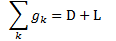
where:

• g_k is the generation from generator k
• D is the total system-wide power demand (sum of individual bus loads
• L is the total transmission losses in the AC network

Starting with this system lambda, each nodal price can be thought of as being made up of these three components:

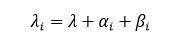
where:

• λ_i is the nodal price
• α_i is the node's congestion charge
• β_i is the node's marginal loss charge

In our 7-Node example the system lambda is the price at the slack bus (Node "1") and is equal to $14.95. In the following section we will show how the prices at the other nodes in the network are calculated from the shift factors and this network energy charge.

3. Congestion Charge

The congestion charge is computed by considering all active transmission constraints and propagating their shadow prices to the nodes using the shift-factors:

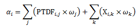
where:

• α_i is the congestion charge at node i
• ω_j is the shadow price on the thermal limit constraints for path j
• X_(i,k) is the angle reference matrix element
• ω_k is the shadow price on the node phase angle constraints for node k

The phase angle could be switched off for some large-scale system simulations. For binding Interface or user-defined constraints the shadow price on the limit is multiplied by the coefficient of the line's flow in the interface definition.

Note that the congestion charge does not need to be positive. For example if the slack bus(es) are located on the high price side of a transmission constraint, the nodes on the low priced side have negative congestion charges.

In our 7-Node Example, there is only one transmission limit with a non-zero shadow price in our economic dispatch and that is for Line "2_5" which has shadow price $10.53. Note that the Line Shadow Price is actually the negative of the shadow price from our LP solution, hence ω_{(2_5)} = -10.53.

The congestion charge at Node "1" is zero because this is the slack bus. To compute the congestion charges in the rest of the network we apply the above formula and shift factors shown in Table 17. For example, for Node "5":

α₅ = -0.5150942 × -10.53 = 5.42

Hence the price at Node "5" is:

λ₅ = λ + α₅ = 14.95 + 5.42 = 22.42

4. Marginal Loss Charge

The marginal loss charge reflects the impact that an increment in nodal injection would have on overall system losses, assuming those losses are absorbed at the slack bus(es). From the optimal solution this is relatively simple to compute:

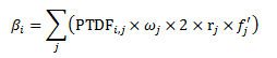
where:

• β_i is the marginal loss charge at node i
• r_j is the resistance on line j
• f'_j is the flow on the line j at the optimal solution

Note that 2 × r_j × f'_j is the marginal loss on line j and is reported as Line Marginal Loss. Although it seems intuitive that these charges should always be positive, they can be positive or negative. For example, if injection at a bus reduces loop flow in the AC network, or provides generation closer to the loads than the optimal solution, then the MLF will be negative. See the 7-Node network for examples.

5. Marginal Loss Factor

The nodal Marginal Loss Factor (MLF), also called a Transmission Loss Factor (TLF), describes what proportion of a one megawatt increment in injection at the node is actually delivered to the slack bus(es) after accounting for incremental transmission losses in the AC network. Unlike shift factors, which are static, the MLF are different for any given set of network injections. PLEXOS reports Node Marginal Loss Factor based on the equation:

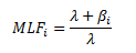
where:

• λ is the system energy charge
• β_i is the marginal loss charge at node i

Note that this equation relies on the nodal energy charge being a non-zero. In the rare case that the system energy charge is zero, a zero MLF is reported.