PLEXOS Stochastic Hydro Optimization
By:
Felipe César Valdebenito Tepper, MSc
Belén Elaine Leveroni Villafana, MSc
Glenn Drayton, Ph.D.
Contents
- Executive Summary
- Introduction
- The Challenge
- The Formulation
- Stochastic Optimization
- Algorithms to solve stochastic hydro-thermal coordination
- Case Study
- Data of the system
- Model solution using SDDP algorithm
- Conclusions
- References
- Annexes
For a PDF version of this article, click the following link:
1. Executive Summary
In decision making under uncertainty, the decision maker has to make optimal decisions throughout a horizon with incomplete information. Over the considered decision horizon, a number of stages are defined and each stage represents a point in time where decisions are made or where uncertainty partially or totally vanishes. According to the number of stages considered in the optimization problem we can distinguish between two-stage and multi-stage stochastic problems. In a two-stage approach, the plan for the entire multi-period planning horizon is determined before the uncertainty is realized, and only a limited number of recourse actions can be taken afterwards. In contrast, a multi-stage approach allows revision of the planning decisions as more information regarding the uncertainties is revealed across the planning horizon.
Regarding stochastic optimization applied to hydro-thermal coordination, the two-stage approach only finds applications for short term operational planning. For medium and long-term studies, a multi-stage stochastic approach is more suitable because, in practice, the system operator or hydro plant companies are monitoring the state of the dam continuously and can take new decisions (stages) at any time given the actual and historical inflow information.
The disadvantage of multi-stage stochastic optimization is that the simulation time increases exponentially when more stages are added due to an increase in the dimensionality of the mathematical problem, and even when a few number of stages are added it can result in a problem impossible to solve without using reduction or decomposition techniques.
To help solve this dimensionality issue some algorithms have been proposed and this paper explores three of them:
- Scenario Reduction
- Stochastic Dual Dynamic Programming (SDDP)
- Hanging Branches
Scenario reduction techniques only finds applications for a few number of stages and a reduced uncertainty, so it is not an option when the user wants to evaluate many stages and increased uncertainty.
SDDP (or DDP) is the method currently used in many countries where hydro-thermal coordination is paramount. It allows the user to evaluate many stages and uncertainty.
The Rolling Horizon method was researched and developed at Energy Exemplar Adelaide's office during 2013 - 2015. The idea behind this method is to formulate the equivalent reduced SDDP multi-stage tree using scenario-wise decomposition techniques plus non-anticipativity constraints.
The comparison table between these three methods is showed below.
| Scenario reduction | SDDP | Rolling Horizon | |
|---|---|---|---|
| Documented in literature? | Yes | Yes | No. Method was developed at Energy Exemplar |
| Recursive vs Non-recursive* | Non-recursive | Recursive | Recursive |
| Multi-stage tree exploration | No resampling | Some SDDP versions resample the tree allowing multiple exploration paths | No resampling |
| Speed solution | An equivalent SDDP tree is impossible to solve using today's available computers | It uses decomposition techniques and parallel resolution of independent sub problems to improve simulation performance. | It should have equivalent speed to SDDP and much faster than scenario reduction. |
| Linear or Integer? | Linear or MIP | Linear Only | Linear or MIP |
| Implemented in PLEXOS? | Yes | No | Yes |
*Non - Recursive: inflow scenarios are revealed after the release policy is taken
The Rolling Horizon method is the method that will ultimately replace SDDP. Initial benchmarks between both methods, documented in this paper, using small multi-stage stochastic trees show that the objective function values are identical. Following the tests shown here more development work was undertaken throughout 2016-17 and the method's results benchmarked against full sized datasets confirming the accuracy of the results.
Additional developments supporting the Rolling Horizon method have been undertaken related to automating the creation of the required hanging branches in the stochastic tree reading historical inflow information. This was necessary because, for large stochastic trees, it is impractical to create a csv file manually with the required uncertainty. The developments undertaken were:
- Historical apertures. Where the hanging branches are created randomly sampling the historical inflow information at each stage.
- PARMA time series. A more powerful option than a) since the hanging branches are be created from past information so, for example, 'wet' observed scenarios are more probably to remain wet in the future. This is achieved using a periodic ARMA time series (PARMA).
2. Introduction
Power systems having both hydro-electric and thermal generation require a systematic and coordinated approach to determine an optimal policy for dam operations. The goal of a hydro-thermal planning tool is to minimize the expected thermal costs across the simulation period. These types of problems generally require stochastic analysis to deal with inflow uncertainty. This can increase the mathematical size of the problem and can easily become cumbersome to solve.
This whitepaper reviews three different algorithms of stochastic programming to solve this problem and how these techniques can be applied to hydro-thermal scheduling problem and introduces the method developed at Energy Exemplar. In addition, a case study solved using SDDP and the proposed method is done and a comparison is provided.
3. The Challenge
The systematic coordination of a system composed of both hydro-electric and thermal plants requires determining an operational strategy that for each period of the planning horizon produces a scheduling plan of generation. This strategy minimizes the expected operational cost along the period, which is mainly composed of fuel costs plus penalties for failure in load supply. The problem becomes complex to solve because generally in hydro systems:
- Natural inflows are stochastic processes.
- Availability of water stored in dams is limited.
- There are complex cascading hydro systems.
- Existing water usage policies and environmental releases such as irrigation settlements.
Water as a fuel supply is cost-free, but its opportunity cost is fundamental to finding the optimal strategy for operations. This issue creates the need for a decision in each time period. Storage cannot be drained too low, which might incur generation shortfalls or excessive thermal output. On the other hand, we also want to avoid spillage of water and lost generation opportunities. Figure 1 summarizes the dilemma a hydro power planner faces to operate a dam.
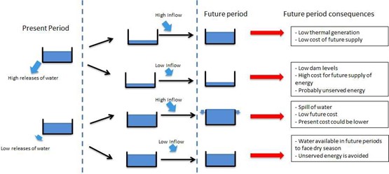 Figure 1: Diagram showing the dilemma hydro power planner faces
under uncertainty.
Figure 1: Diagram showing the dilemma hydro power planner faces
under uncertainty. 4. The Formulation
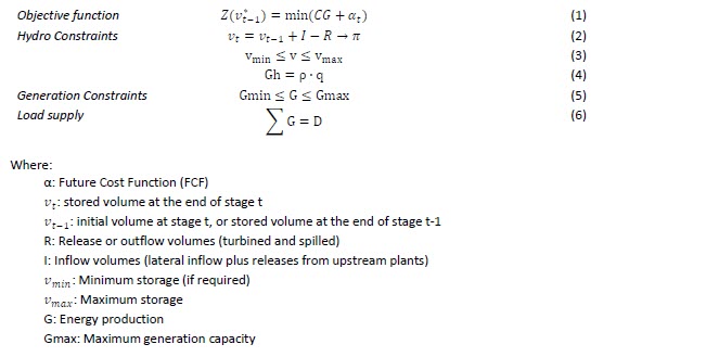
A mathematical optimization tool can find a hydro releasing policy that minimizes the expected operational thermal cost by formulating an optimization problem such as the following:
Where the hydro balance equation shows the link between decisions in both the present and future.
Since water is free (no fuel cost) it is necessary to specify a final condition to minimise thermal costs along the simulation period, and to avoid the storage being completely drained. These final conditions can be represented as a target or a proxy for opportunity costs such as a deviation from targets, usually known as the future cost function or scrap value function.
5. Stochastic Optimization
In decision making under uncertainty, the decision maker must make optimal decisions throughout a decision horizon with incomplete information. Over the considered decision horizon, many stages are defined and each stage represents a point in time where decisions are made or where uncertainty partially or totally vanishes. The amount of information available to the decision maker is usually different from stage to stage. According to the number of stages considered in the optimization problem we can distinguish between:
- Two-stage stochastic problems
- Multi-stage stochastic problems
The stochastic problem is graphically represented as a scenario tree.
5.1. Scenario Tree Representation
A scenario tree consists of nodes and lines grouped in stages as showed in Figure 2. Each node in the scenario tree represents a possible state and it is a point in time where decisions are made.
The lines in the scenario tree are called "leaves" and represents the possible outcomes for the random variables so each of them has a probability associated. The sum of probabilities associated to each node is unity.
A path from the root node to any other node describes one realization of the stochastic process from the present time to the period that node appears. A path over the entire planning horizon is called a scenario.
Figure 2 shows a scenario tree consisting of 15 nodes, eight scenarios and three stages. This scenario tree represents a decision-making process where the decisions are re-evaluated four times (three stages plus the root node) along the planning horizon according to the revealed information at each stage.
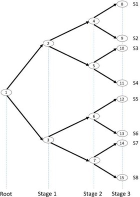 Figure 2: Scenario Tree representation
5.1.1. Two-stage Stochastic Problem
Two-stage applies to a decision-making problem where decisions are made in two stages and there exists uncertainty represented by a set of scenarios or samples. It can be assumed that two different decision variable vectors: x and y are involved in this problem. Decision x is made before knowing the actual value of the scenarios, while y is determined after knowing the actual value of the scenario.
Decision y depends on the decision x previously made. The decision-making process is as follows:
- Decision x is made
- The uncertainty is revealed
- Decision y is made
In this decision-making process, two kinds of decision are made:
- First-stage or 'here-and-now' decisions (Decision x). These decisions are made before the realization of the stochastic process. Hence, variables representing here-and-now decisions do not depend on each realization of the stochastic process.
- Second-stage or 'wait-and-see' decisions (Decision y). These decisions are made after knowing the actual realization of the stochastic process. Consequently, these decisions depend on each realization vector of the stochastic process. If the stochastic process is represented by a set of scenarios, a second stage decision variable is defined for each single scenario considered.
For all these decisions to be optimal, they need to be derived simultaneously by solving a single optimization problem, so that the relationships among the decision variables are properly accounted for.
5.1.2. Multi-stage Stochastic Problem
In some cases, decision-making problems have more than two stages, and the two-stage stochastic programming problem showed above is not appropriate to represent them. This fact motivates the use of multi-stage stochastic programming problems. The decision-making process for a multi-stage stochastic problem with r stages is the following:
- Decisions x1 are made
- Partial uncertainty is revealed
- Decisions x2 are made
- Partial uncertainty is revealed
- Decisions x3 are made
...
2r-2. Uncertainty is revealed
2r-1. Decision xr are made
This decision framework for a multi-stage problem is conveniently visualized using a scenario tree diagram like the tree in Figure 2.
5.2. Stochastic Problem Formulation: Two-stage vs Multi-stage
In a two-stage approach, the plan for the entire multi-period planning horizon is determined before the uncertainty is realized, and only a limited number of recourse actions can be taken afterwards. In contrast, a multi-stage approach allows revision of the planning decisions as more information regarding the uncertainties is revealed along the planning horizon. Consequently, the multi-stage model is a better characterization of the dynamic planning process, and provides more flexibility than does the two-stage model.
Figure 3 shows an expected comparison when the same optimization problem is solved using simple average deterministic, two-stage stochastic optimization, and multi-stage stochastic optimization. As can be observed, the expected cost is lower in a multi-stage problem when the number of stages increases because the decision maker has opportunity to re-evaluate his initial decision as additional information arrives.
The disadvantage of multi-stage stochastic optimization problems is that the dimensionality increases exponentially when more stages are added and even when a few number of stages are added it can be impossible to solve without using reduction or decomposition techniques because of large dimensionality resulting problems.
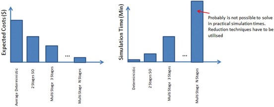 Figure 3: Comparison between expected costs and simulation times
solving the problem in deterministic, 2 stages and multi-stage
Figure 3: Comparison between expected costs and simulation times
solving the problem in deterministic, 2 stages and multi-stage
Regarding stochastic optimization applied to hydro-thermal coordination, the two-stage approach only finds applications for short term operational planning. For medium and long-term studies, a multi-stage stochastic approach is more suitable because, in practice, the system operator or hydro plant companies are monitoring the state of the dam continuously and can take new decisions (stages) at any time given the actuals and historical inflow information.
5.3. Stochastic Problem Formulation: Node vs Scenario-wise Decomposition
A stochastic programming problem can be mathematically formulated using either a node-variable formulation or a scenario-variable formulation. The first formulation relies on variables associated with decision points while the second one relies on variables associated with scenarios.
Consider the example summarized in Figure 4 which shows a multi-stage stochastic problem where at each stage there are two possible outcomes for the inflow: Wet and Dry.
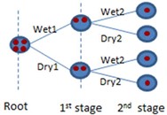 Figure 4: Scenario tree
5.3.1 Node formulation
The node-variable formulation of this problem is as follows:
P) Min {C1(R11) + p21[C2(R21) + p31C3(R31) + p32C3(R32)] + p22[C2(R22) + p33C3(R33) + p31C3(R31)]}
Subject to:
- V11 = V01 - R11 + /11
- V21 = V11 - R21 + /21
- V31 = V21 - R31 + /31
- V32 = V21 - R32 + /32
- V22 = V11 - R22 + /22
- V33 = V22 - R33 + /33
- V34 = V22 - R34 + /34
- Energy Balance
- Storage Capacity
- Max Capacity
Where:
- Vi,k: End volume at stage i, scenario k
- Ri,k: Storage release at stage i, scenario k
- /i,k: Inflow at stage i, scenario k
- pi,k: Probability of scenario k at stage i.
- C(Ri,k): Thermal cost that results from release policy Ri,k
5.3.2 Scenario-wise Decomposition (SWD) or scenario-variable formulation
The Scenario-wise Decomposition formulation of this problem is as follows:
P) Min {p11×p21[C1(R11)+C2(R21) + C3(R31)] + p11×p22[C1(R12)+C2(R22) + C3(R32)] + p12×p21[C1(R13)+C2(R23) + C3(R33)] + p12×p22[C1(R14)+C2(R24) + C3(R34)]}
Subject to:
- V11 = V01 - R11 + /11
- V21 = V11 - R21 + /21
- V31 = V21 - R31 + /31
- V12 = V02 - R12 + /12
- V22 = V12 - R22 + /22
- V32 = V22 - R32 + /33
- V13 = V03 - R13 + /14
- V23 = V13 - R23 + /24
- V33 = V23 - R33 + /34
- V14 = V04 - R14 + /14
- V24 = V14 - R24 + /24
- V34 = V24 - R34 + /34
- Energy Balance
- Storage Capacity
- Max Capacity
- V01=V02=V03=V04
- V11=V12=V13=V14
- V21=V22
- V23=V24
- V31, V32, V33, V34 free
Where:
- Vi,k: End volume at stage i, scenario k
- Ri,k: Storage release at stage i, scenario k
- /i,k: Inflow at stage i, scenario k
- pi,k: Probability of scenario k at stage i.
- C(Ri,k): Thermal cost that results from release policy Ri,k
Scenario-wise decomposition requires a larger number of variables and constraints including those marked in blue above called "non-anticipativity". These conditions guarantee that decisions cannot be dependent on the scenario realization. They are logical constraints related to availability of information at any decision point in time. Red circles in Figure 4 shows non-anticipativity variables that need to be enforced at each node.
5.4. Recourse vs Non-recursive Multi-stage Stochastic Problem
The decision model should be designed to allow the user to adopt a decision policy that can respond to events as they unfold. To formulate a multi-stage problem with dynamic stochastic data during time, emphasis has to be placed on the decision to be made today, given present resources, future uncertainties and possible recourse actions in the future.
Depending on the availability of information on the uncertain parameters at the beginning of each stage in the scenario tree, different recourse actions are defined for them.
It is possible to identify two types of decision depending on the availability of the information at the beginning of each stage:
- Recursive: At the beginning of each stage, the
decision maker has a perfect insight on the inflow scenario that
will be observed at that stage. Thus, the decisions can be adjusted
for different inflow scenarios.
- Non-recourse: If inflow scenario values are revealed after the release policy is taken.
5.4.1. Recursive multi-stage
The recursive multi-stage can be represented in the following scenario tree Figure:
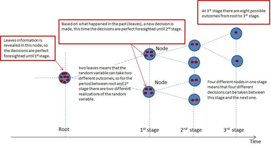 Figure 5: Scenario tree for recursive multi-stage
5.4.2. Non - Recursive multi-stage
The non - recursive multi-stage can be represented in the following scenario tree Figure:
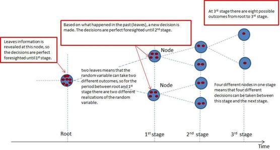 Figure 6: Scenario tree for non-recursive multi-stage
 The scenario tree representation doesn't say if the multi-stage problem is recursive or non-recursive so in addition to the diagram it is necessary to specify what type of recourse actions are available.
The following figure compares both approaches applied to stochastic multi-stage hydro problems where end volumes have to be decided given uncertainty in future inflows.
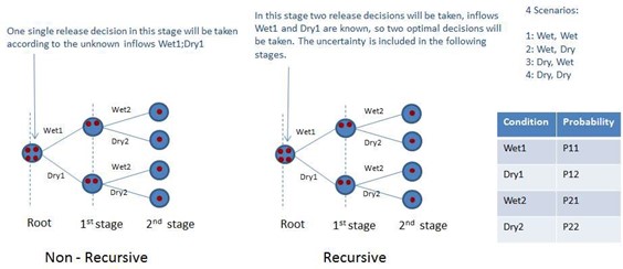 Figure 7: Recursive vs non-recursive multi-stage stochastic
problems
Figure 7: Recursive vs non-recursive multi-stage stochastic
problems
5.5. Stochastic multi-stage hydro dimensionality issue
When using multi-stage stochastic optimization, many possible scenarios can be generated as shown in Figure 8. For such a high number of scenarios, it is impossible to numerically obtain a solution for the multi- stage optimization problem. Different techniques have been introduced in the literature to help solve this problem and commonly involve scenario tree reduction or a more simplified tree solved with decomposition techniques.
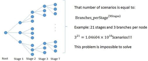 Figure 8: Multi-stage dimensionality issue
 6. Algorithms to solve stochastic hydro-thermal coordination
6.1. Multi-stage tree reduction
PLEXOS implements scenario reduction techniques as an option for solving these problems. These techniques use strategies to reduce the number of scenarios in the optimization problem using algorithms for constructing a multi-stage scenario tree out of a given set of scenarios.
Since generating a very small number of scenarios by Monte Carlo simulation is not desired because less scenarios give less information, the objective is to lose minimum information by the reduction process applied to the complete set of scenarios.
The disadvantage of this technique is that it is necessary to reduce the tree to a very small tree to make it mathematically solvable by current solvers. In most real cases, the resultant tree doesn't represent the uncertainty well.
6.2. Stochastic Dual Dynamic Programming
Stochastic Dual Dynamic Programming (also called simple "Dual Dynamic Programming") is a method developed in the 1970s (Read, 1979) where the hydro temporal coupling decisions are broken and replaced by the concept called the Future Cost Function.
The hydro problem at each stage becomes:
An iterative approach is needed to create the Future Cost Function with cuts that approximate the real future cost function with a piecewise linear function (see Figure 10) that samples the storage at "interesting" states. One cut is created at each iteration and the method stops when a convergence criterion is met.
6.2.1. Schematic representation of SDDP
The multi-period stochastic hydro problem can be decomposed in multiple steps where each step can be represented by the sum of:
- Actual cost: Corresponds to the thermal variable generation costs in that step.
- Future cost: Corresponds to the future thermal variable generation costs associated to the future steps.
At each step, the corresponding actual costs decrease if more water is used but future costs increase so there is an optimal point where the release decision minimizes the sum of actual and future costs.
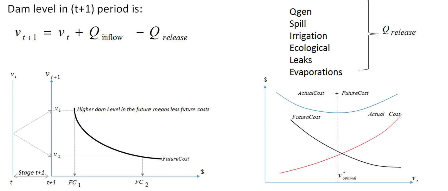 Figure 9: Actual and future costs schematic
representation
Figure 9: Actual and future costs schematic
representation Each step is modelled as a linear programming (LP) problem and the iterative procedure has two passes: forward and backward. One cut for the future cost function at that particular step is created in each backward pass.
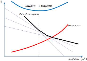 Figure 10: Future cost function approximation
The algorithm to build the approximations to the Future Cost Function is summarized in the following section.
6.2.2. SDDP Algorithm
class="ui image" src="assets/images/Article/Article.PLEXOSStochasticHydroOptimization/SDDP%20Algorithm_1.jpg" width="600">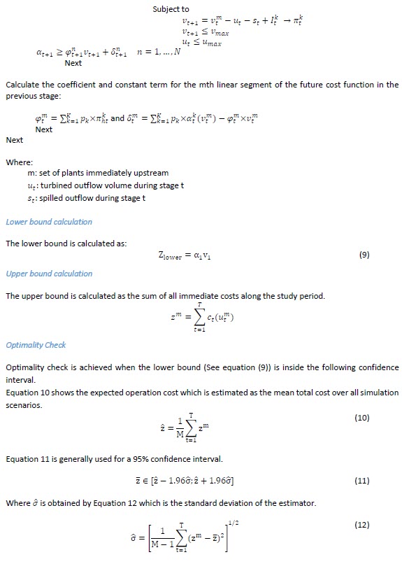
6.2.3. Solving the full multi-stage stochastic graphically tree using SDDP
The SDDP algorithm can be explained graphically using the following multi-stage tree:
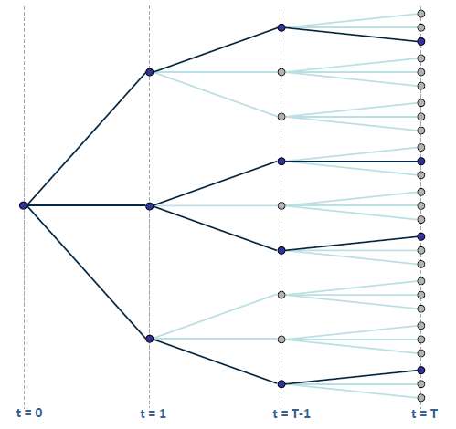 Figure 11: Full multi-stage tree to be solved
using SDDP algorithm
Figure 11: Full multi-stage tree to be solved
using SDDP algorithm Blue paths are the forward simulation paths and light blue are the paths representing uncertainty, these light blue paths are used in the backward pass.
Forward Pass
The forward pass can be summarized in the following figures, where the problem is decomposed in steps with a duration coincident with stage duration and the link between stages is represented using a Future Cost Function (FCF).
The first step mathematical problem can be represented using the following diagram:
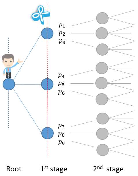 Figure 12: First step SDDP forward simulation,
sub problem 1
Figure 12: First step SDDP forward simulation,
sub problem 1 The second step mathematical problems can be represented using the following diagrams:
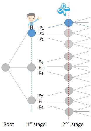 Figure 13: Second step SDDP forward simulation,
sub problem 2
Figure 13: Second step SDDP forward simulation,
sub problem 2 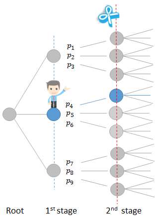 Figure 14: Second step SDDP forward simulation,
sub problem 3
Figure 14: Second step SDDP forward simulation,
sub problem 3 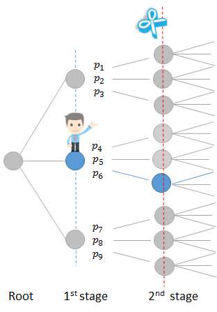 Figure 15: Second step SDDP forward simulation,
sub problem 4
Figure 15: Second step SDDP forward simulation,
sub problem 4 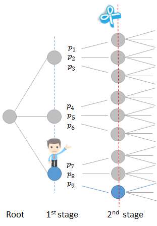 Figure 16: Second step SDDP forward simulation,
sub problem 5
Figure 16: Second step SDDP forward simulation,
sub problem 5 The sub-problems are independent and sub problems in same step can be run in parallel.
The third step is similar.
Backward Pass
The backward pass at each stage can be summarized in the following figures, where the yellow branches are the independent problems solved at each stage. Each backward stage produces a new cut to calculate the FCF.
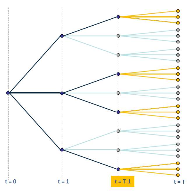 Figure 17: SDDP backward pass and FCF
approximation at t=T-1
Figure 17: SDDP backward pass and FCF
approximation at t=T-1 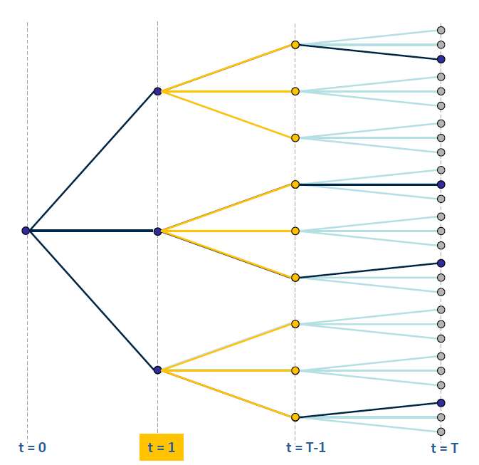 Figure 18: SDDP backward pass and FCF
approximation at t=1
Figure 18: SDDP backward pass and FCF
approximation at t=1 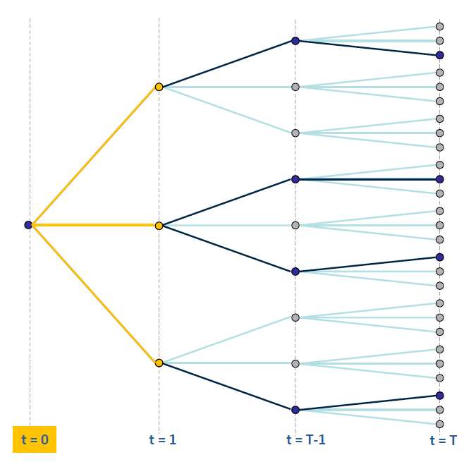 Figure 19: SDDP backward pass at t=0
 It can be observed that all nodes of the forward and backward pass are solved independently.
Simplified tree solved using SDDP
SDDP algorithm can be formulated to solve the full multi-stage stochastic tree but it has the same dimensionality issue described in Figure 8, where the number of sub-problems are equal to: LeavesNumberStages.
The simplified SDDP tree reduces the size of the problem and then become mathematically solvable. This reduced tree has the following number of subproblems: Leaves x NumberStages. The following figure summarizes this simplified tree where red paths are the paths explored during forward simulation and grey branches represent uncertainty at each stage.
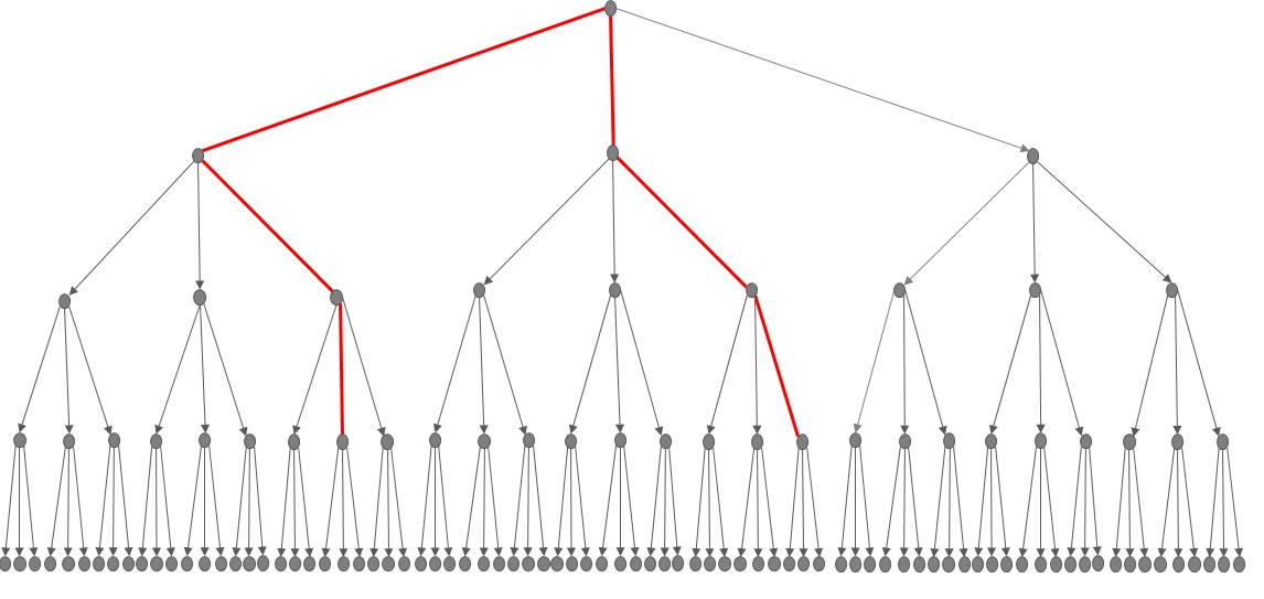
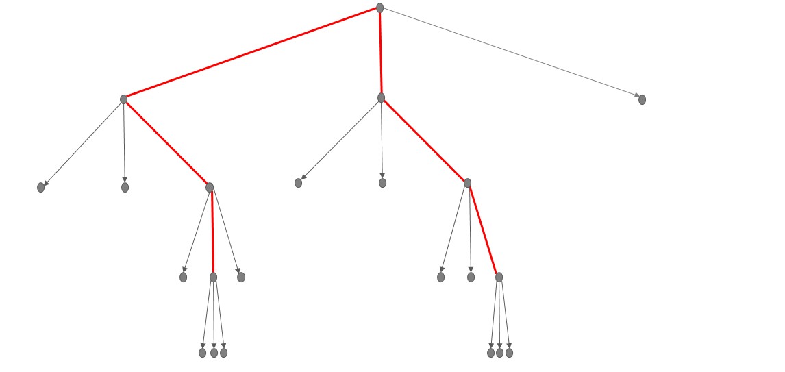 Figure 20: Full tree vs SDDP tree
6.3. Hanging branches
This method was researched and developed at Energy Exemplar's Adelaide office during 2013-2015. The problem is formulated using recursive scenario-wise decomposition formulation and the SDDP stochastic tree.
The full tree can be classified in full branches, hanging branches and death branches as showed below:
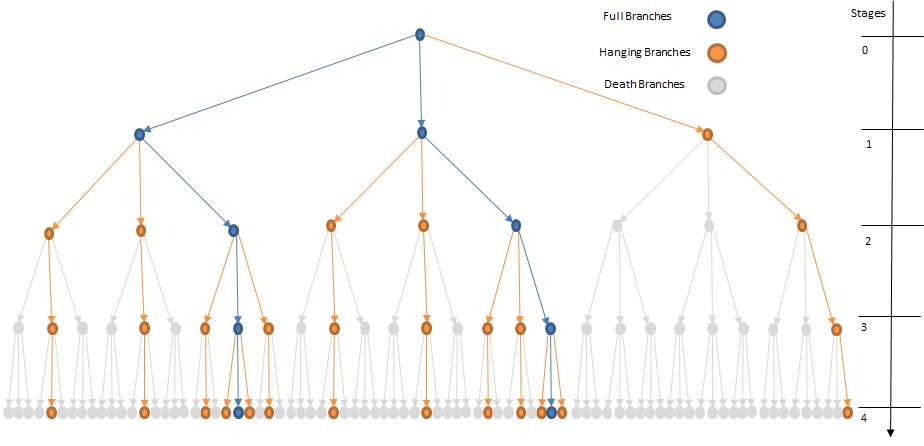 Figure 21: Full multi-stage tree illustrating
full, hanging and death branches
Figure 21: Full multi-stage tree illustrating
full, hanging and death branches The resulting tree to be formulated in an optimization problem is:
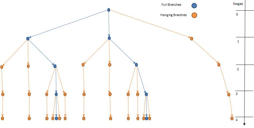 Figure 22: Reduced multi-stage tree illustrating
the equivalent tree.
Figure 22: Reduced multi-stage tree illustrating
the equivalent tree. As in SDDP, this method formulates a full recursive multi-stage stochastic problem. This method in PLEXOS is defined using the Global class of objects as showed in figure below:
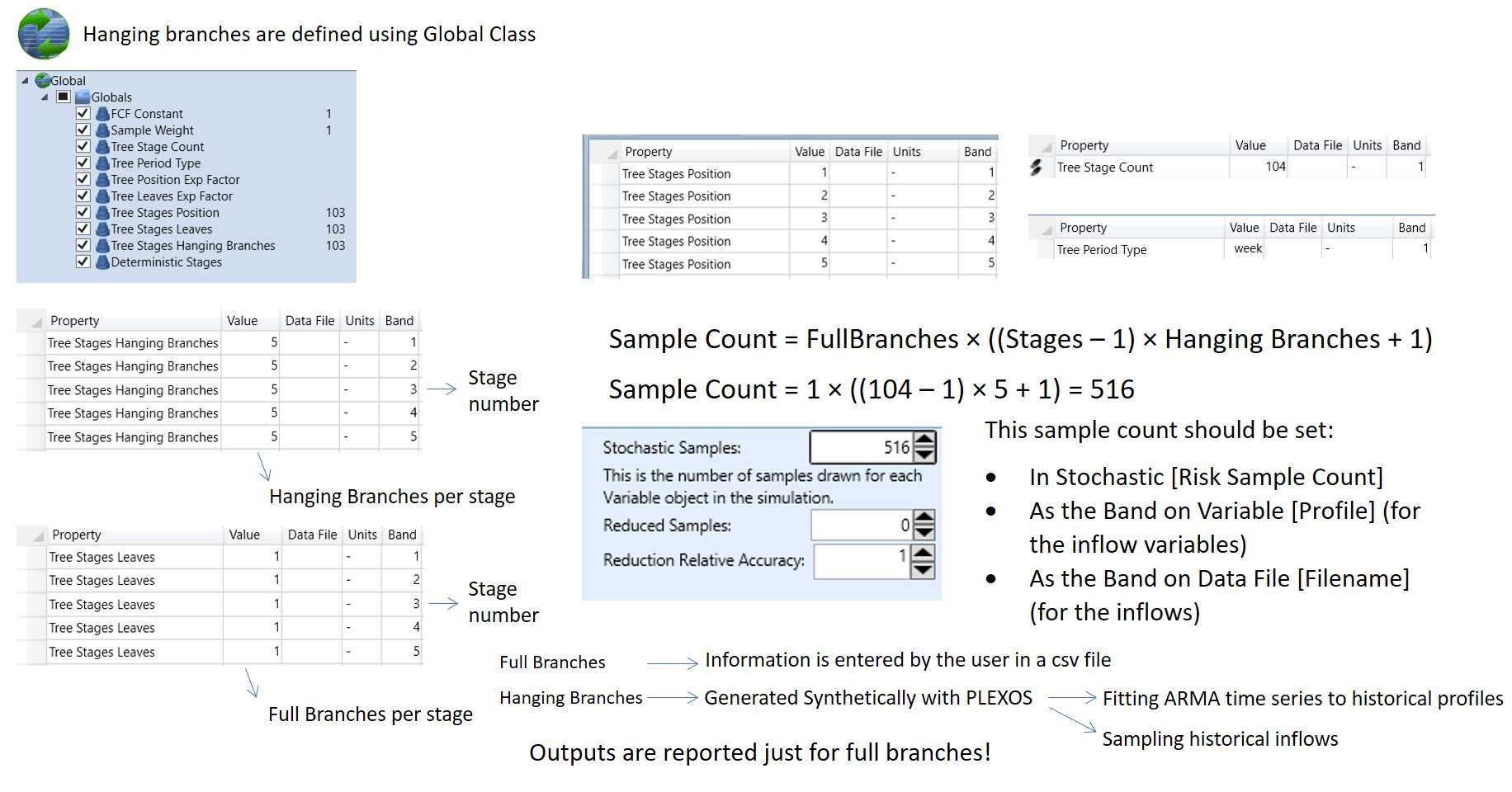 Figure 23: Hanging branches implementation in PLEXOS for 2 years
horizon, 5 hanging branches and 1 full branch per stage and stages
placed at the end of each week.
Figure 23: Hanging branches implementation in PLEXOS for 2 years
horizon, 5 hanging branches and 1 full branch per stage and stages
placed at the end of each week. To help to improve the speed, the hanging branches were designed to have one block per stage from the stage that follows the stage they were created. This is like the equivalent SDDP reduced tree showed in Figure 20.
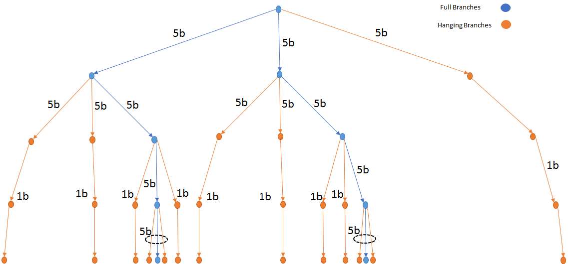 Figure 24: First stage of hanging branches have a
block duration equal the blocks specified and the further stages are
reduced to 1 block. This example is showing the reduction when the
user specifies 5 blocks LDC.
Figure 24: First stage of hanging branches have a
block duration equal the blocks specified and the further stages are
reduced to 1 block. This example is showing the reduction when the
user specifies 5 blocks LDC. 6.3.1. Hanging branch weights
When the hanging branches equivalent multi-stage tree is formulated, it exists a solver limitation to solve the problem in one single step.
For example, if the user would like to solve this problem: 120 stages, 40 hanging branches per stage and 40 full branches for 10 years using 5 blocks LDC per month. This means the following:
- The first 41 branches (40 hanging + 1 full branch) has 1/41 probability occurrence.
- The second stage has 41 branches (40 hanging + 1 full branch) so each one has 1/41 probability of occurrence. So, from the first stage the probability for each second stage branch is 1/41*1/41.
- For next stages it is the same.
Then solving the problem from the first stage until the last one produces tiny weights for future branches, this is illustrated in the table below for the example described above:
| Stage Number | Probability | Probability |
|---|---|---|
| 1 | 1/41 | 0.024390244 |
| 2 | (1/41)^2 | 0.000594884 |
| 3 | (1/41)^3 | 1.45094E-05 |
| 4 | (1/41)^4 | 3.53887E-07 |
| 5 | (1/41)^5 | 8.63139E-09 |
| 6 | (1/41)^6 | 2.10522E-10 |
| 7 | (1/41)^7 | 5.13468E-12 |
| 8 | (1/41)^8 | 1.25236E-13 |
| 9 | (1/41)^9 | 3.05454E-15 |
| 10 | (1/41)^10 | 7.45009E-17 |
| 11 | (1/41)^11 | 1.81709E-18 |
| 12 | (1/41)^12 | 4.43194E-20 |
| 13 | (1/41)^13 | 1.08096E-21 |
| 14 | (1/41)^14 | 2.63649E-23 |
| 15 | (1/41)^15 | 6.43046E-25 |
| 16 | (1/41)^16 | 1.56841E-26 |
| 17 | (1/41)^17 | 3.82538E-28 |
| 18 | (1/41)^18 | 9.33019E-30 |
| 19 | (1/41)^19 | 2.27566E-31 |
| ... | ... | ... |
A safe range of objective coefficients guaranteed by a commercial solver is between 10^-6 and 10^6, that means it can only be ensured a multi-stage solution until stage three.
The multi-stage stochastic optimization says that at each stage the decision maker can change his mind and take a new decision because additional information is revealed, so this limitation can be solved in the same way a multi-stage stochastic problem is solved in the real life: using a rolling horizon approach splitting the horizon in steps. The only information passed between steps is related to storage end/initial volumes.
6.3.2. Hanging branches with rolling horizon
The Rolling Horizon approach is designed to overcome the limitation of vanishingly small probabilities deep into the future. The method looks ahead until certain point in the future and the end volumes in that point are passed as initial volumes at the start of the next step.
For a horizon divided in four different steps, the algorithm works as follows:
Step 1:
- Starting date is beginning of root node.
- Multi-stage tree formulated and up to some stage in the future (user decides when) no more branches to avoid weights issue.
Step 2:
- Starting date is beginning of stage 1.
- End volumes in step 1 are passed as initial volumes in step 2.
- The past branches are not formulated because that part of the problem is already solved.
Step 3:
- Starting date is beginning of stage 2.
- End volumes in step 2 are passed as initial volumes in step 3.
- The past branches are not formulated because that part of the problem is already solved.
- More hanging branches are formulated when the weights provide information to the optimization solver.
Step 4:
- Starting date is beginning of stage 3.
- End volumes in step 3 are passed as initial volumes in step 4.
- The past branches are not formulated because that part of the problem is already solved.
- The problem becomes a simple deterministic problem since no more uncertainty is added because it is a recursive multi-stage problem.
Figure 25 shows the hanging branches method for a multi-stage problem consisting of 4 stages, 2 hanging branches per stage and 1 full branch where the horizon is divided in 4 different steps.
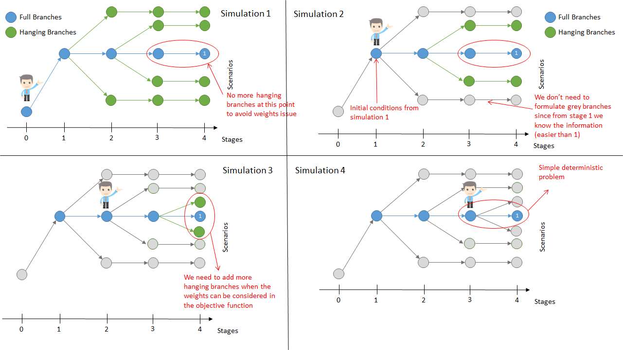 Figure 25: Rolling horizon for hanging branches
6.4. Comparison of different stochastic programming algorithms
Table 2 summarizes the difference between the three methods studied: scenario tree reduction, SDDP and Rolling Horizon approach to solve stochastic multi-stage problems.
| Scenario reduction | SDDP | Rolling Horizon | |
|---|---|---|---|
| Documented in literature? | Yes | Yes | No. Method was developed at Energy Exemplar |
| Recursive vs Non Recursive | Non Recursive | Recursive | Recursive |
| Multi-stage tree exploration | No resampling | Some SDDP versions resample the tree allowing multiple exploration paths | No resampling |
| Speed solution | An equivalent SDDP tree is impossible to solve using today's available computers | It uses decomposition techniques and parallel resolution of independent sub problems to improve simulation performance. | It should equivalent to SDDP but faster than scenario reduction. |
| Linear or Integer? | Linear or MIP | Linear Only | Linear MIP |
| Implemented in PLEXOS? | Yes | No | Yes |
7. Case Study
Click the link below to view a case study showing the resolution of the problem using SDDP and hanging branches method.
 CASE STUDY: PLEXOS Stochastic Hydro
Optimization using SDDP and hanging branches method
CASE STUDY: PLEXOS Stochastic Hydro
Optimization using SDDP and hanging branches method
7.2. Model solution using SDDP algorithm
8. Conclusions
The approach to solve hydro-thermal coordination optimization
problems is to use stochastic optimization techniques to ensure the
user minimizes the cost or alternatively maximizes the benefits of a
hydro-thermal portfolio under uncertainty. A stochastic problem can be
classified in:
- Two-stage or Multi-stages
- Recursive or non-recursive
The formulation of a multi-stage stochastic problem has dimensionality issues even when a few number of stages are added so simplifications on the resultant tree have to be made to produce a problem solvable by today computers.
An equivalent SDDP tree is possible to formulate using scenario-wise decomposition and nonanticipativity constraints. This problem is possible to solve using today's computers.
The Rolling Horizon method in looks promising to replace SDDP.
9. References
A multi-stage stochastic programming approach for production planning with uncertainty in the quality of raw materials and demand. ZanjaniM.K.,Nourelfath, M. / Ait-Kadi, D.16, International Journal of Production Research, 4701-4723.
ConejoA.J.,Carrión, M. & Morales, J.M. Decision Making Under Uncertainty in Electricity Markets. Boston, MA, Springer U.S., 2010.
NewhamN. Power System Investment Planning using Stochastic Dual Dynamic Programming. 2008.
ReadE.Grant Power System Optimisation. , University of Canterbury, 1979.
Stochastic Dual Dynamic Programming with CVar Risk Constraints Applied to Hydrothermal Scheduling . Da Costa JuniorPereira,Granville, Campodónico, Costa Fampa2013. International Conference on Stochastic Programming.
Stochastic optimization of a hydro-thermal system including network constraints. al.Pereiraet2, IEEE Transactions on Power Systems, 791-797.
TroncosoC. Herramienta docente para estudios de coordinación hidrotérmica. 2010.
10. Annexes
SDDP algorithm deterministic approach
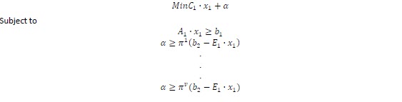
Benders cuts take advantage of the following mathematical structure:

This can be interpreted as a two-stage sequential decisions process. In the first stage we decide on a trial feasible value for X1 and given the trial value we find the optimal solution of the second stage function:

X1 is known value in the second stage problem, and goes to the right hand side of the constraints. The objective then is to minimize the sum of the first - stage and second stage cost functions:

Where C1X1 represents the "actual cost" and α represents the "future cost" of decision X1. The future cost function translates the second stage costs as a function of the first stage decisions X1. If this function is available the problem can be solved as a one stage problem and then simplify the computation time.
The future cost function is approximated by an analytical function rather than a set of discrete values using a piecewise linear function. The structure of the future cost function can be characterized by taking the dual of the second stage problem:

π is the row vector of dual variables. From LP theory, optimal solution of dual and the original problem coincide. Since X1 is in the objective function and not in the right hand side of the constraint set as in the original problem, the set of possible solutions can be characterized before knowing the decision X1.
The problem can be solved by enumeration:

This is equivalent to rewrite the problem as:

The problem can be rewritten as:
We can rewrite the obtained cuts:
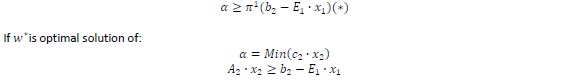
Assuming dual and primal has the same value we can write:

Substituting previous expression in cuts formulation (*), we can get an alternative expression for FCF:

Hydro problems share same mathematical structure described above where the link between stages is the hydro balance equation:

SDDP algorithm stochastic approach:
Stochastic problems can be written as:
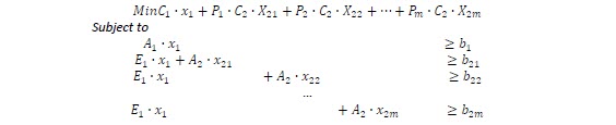
Were p1 and p2 are the probabilities to obtain b1 and b2. The second stage problem can be written as follows:

This problem can be decomposed into two independent problems:

The original problem can be rewritten as:

The function α represents expected value of future cost function:

The benders cuts associated to this problem are:

That can be rewritten as:

Grouping the above equation we obtain the cut expression for stochastic problems:
