Pumped Storage
Contents
- Introduction
- Creating a Pumped Storage
- Initial Volume
- End Period Storage Volume
- Decomposition and Step Size
- Technical Constraints
- Pumped Storage Example
1. Introduction
Pumped storage plants store energy in the form of water, pumped from a lower elevation reservoir (the 'tail' storage) to a higher elevation ('head' storage). Low-cost off-peak electric power is used to run the pumps. During periods of high electric demand (and high price), the stored water is released through turbines to generate power. Although the losses of the pumping process make these plant a net consumer of energy overall, the system benefits from the arbitrage of cheap off-peak generation into the more expensive on-peak.
2. Creating a Pumped Storage
There is no specific 'type' setting for pumped storage hydro plant. Instead pumped storage is modelled using the Generator class and are identified by their unique data:
- Pump Load
- Pump Load is the megawatt load drawn from units in pumping mode.
- Pump Efficiency
- Pump Efficiency is the round-trip percentage efficiency of the pumped storage plant. For example an efficiency of 75% implies that for every unit of generation then 1/0.75= 1.3333 units of energy are required to pump the required water back to the head storage. Further this implies that the price received when generating must be at least 33.33% higher than the price paid for pump energy.
These two properties identify the Generator as a pumped storage, but you must also model the connected storages. Thus two Storage objects are required:
- one for the Generator Head Storage; and
- one for the Generator Tail Storage.
You need only define the Storage Max Volume on these storages. The following tables show a simple pumped storage plant and the required memberships between the Generator and the Storage objects.
| Name | Property | Value | Units |
|---|---|---|---|
| Pumped Hydro | Units | 1 | - |
| Pumped Hydro | Max Capacity | 1000 | MW |
| Pumped Hydro | Pump Load | 1000 | MW |
| Pumped Hydro | Pump Efficiency | 75 | % |
| Collection | Parent Name | Child Name |
|---|---|---|
| Generator.Head Storage | Generator (Pumped Hydro) | Storage (Pumped Head) |
| Generator.Tail Storage | Generator (Pumped Hydro) | Storage (Pumped Tail) |
| Name | Property | Value | Units |
|---|---|---|---|
| Pumped Head | Max Volume | 30 | GWh |
| Pumped Tail | Max Volume | 30 | GWh |
The data in Tables 1 through Table 3 defines the pumped storage system
illustrated in Figure 1. The left-hand diagram shows the generation
cycle and how this affects the storages and the injection to the
network. Likewise the right-hand diagram shows the pump cycle: note
the effect of the efficiency such that a one megawatt load results in
0.75 megawatt-hours of potential energy pumped to the head storage.
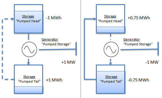 Figure
1: Pumped storage cycle
Figure
1: Pumped storage cycle
3. Initial Volume
By default, the head storage will be assumed full, and the tail empty in the first hour of the simulation. You may override this using the Storage Initial Volume property of the head and tail storages as in Table 4.
| Name | Property | Value | Units |
|---|---|---|---|
| Pumped Head | Max Volume | 30 | GWh |
| Pumped Head | Initial Volume | 25 | GWh |
| Pumped Tail | Max Volume | 30 | GWh |
| Pumped Tail | Initial Volume | 5 | GWh |
4. End Period Storage Volume
The method used to value end-of-period storage is controlled by the Storage End Effects Method
attribute. The default setting depends on whether or not the pumped
storage is considered a 'simple' pumped system i.e. one that
is not part of a cascading river network.
Note: A cascade is a network of more than one interconnected
storage.
For 'simple' pumped storage systems, by default, the Storage
End Effects Method for the
head storage is "Recycle", which means the head storage level will
return to its starting position at the end of each simulation step;
and in a closed loop system like this it also implies that the tail
storage will return to its starting level.
Pumped storages that are part of cascading systems are treated the
same as 'normal' storages and follow the rules shown in the article Cascading Hydro Networks
which means you should set the Storage End Effects Method if the
default is not appropriate.
5. Decomposition and Set Size
Pumped storage release and pumping decisions are not decomposed by MT Schedule, which means their
operation is independently optimized by ST
Schedule.
The reason for this is the load-duration curve model in MT
Schedule does not (in general) capture the peak to off-peak
price differentials that the full chronological model does, and thus
it tends to understate the utilization of pumped storage. Thus the
simulator leaves the optimization of pumped storage 'free' for ST
Schedule.
This has important implications for the chronological model's step
size. If the ST Schedule step size
is short (e.g. a day at a time) then arbitrage opportunities might be
missed. It is normal practice then to model sufficient look-ahead in ST Schedule that the pumped storages
can arbitrage across each week. This is achieved either through a
weekly step size in ST Schedule,
or if that is not feasible computationally, then a daily step with
additional days of look-ahead (potentially at a lower than hourly
resolution).
6. Technical Constraints
Pumped storage can be subject to a number of technical limitations. Table 5 outlines the input properties available to model these constraints.
| Property | Unit | Constraint modeled |
| Pump Units | - | Not all Units at the Generator are capable of pumping |
| Min Pump Load |
MW |
The pumping operation cannot be performed at loads below a
certain level |
| Must Pump Units |
- |
The pumping schedule is fixed for at least some periods of
time |
| Max Units Pumping |
- |
There is limit on the number of Pump Units units that can pump
in some periods of time |
| Fixed Pump Load |
MW |
There is a given fixed pumping schedule for at least some
periods of time |
| Min Pump Time | h | There is a minimum running time for any pumping operation block |
| Min Pump Down Time | h | There is a minimum time between pumping operation blocks |
| Generation Transition Time | h | There is a minimum time required between generation and pumping operation blocks |
| Pump Transition Time | h | There is a minimum time required between pumping and generation operation blocks |
7. Pumped Storage Example
Returning to our hydro-thermal coordination problem: assume now that insert the pumped storage plant defined in the above tables in place of the energy-constrained and/or simple storage driven hydro plant.
Case 5
Pumped storage with daily step:
In this case we run ST Schedule
alone with a step size of a day, meaning that the year-long horizon is
solved in 365 steps each of 24 hours. The results are shown in Table
6. Note that the total Energy increases due to the pump load, but
overall there are net savings on thermal cost.
| Property | Energy | Price | Generation | Thermal Cost | Savings (Case 0 - Case 5) |
|---|---|---|---|---|---|
| Units | GWh | $/MWh | GWh | 0 | 0 |
| Jan | 851 | 53 | 851 | 33314 | 16 |
| Feb | 648 | 47 | 648 | 24414 | 2 |
| Mar | 722 | 48 | 722 | 27213 | 3 |
| Apr | 839 | 53 | 839 | 33061 | 18 |
| May | 1078 | 66 | 1078 | 45944 | 189 |
| Jun | 1267 | 88 | 1267 | 60410 | 998 |
| Jul | 1445 | 111 | 1445 | 74532 | 2933 |
| Aug | 1412 | 107 | 1412 | 71292 | 2358 |
| Sep | 1230 | 85 | 1230 | 57423 | 771 |
| Oct | 1034 | 63 | 1034 | 43595 | 127 |
| Nov | 794 | 51 | 794 | 31016 | 14 |
| Dec | 713 | 47 | 713 | 26872 | 2 |
| Total | 12033 | 74 | 12033 | 529086 | 7431 |
Case 6
Pumped storage with weekly step:
This case is the same as Case 5 but ST
Schedule is configured to solve in weekly steps. In fact because
weeks do not fit neatly into a year we are running 53 weeks and
'discarding' the results for the last few days. The results for this
case are shown in Table 7. Comparing these to Case 5, the weekly step
size greatly improves the utilization of the pumped storage; in fact
the capacity factor for the generator increases from 1.9% to 7.92%.
Figure 11 compares a month of hourly pumped storage head storage
volumes, and this shows very clearly the greatly increased utilization
of the pumped storage in the weekly ST
Schedule case.
In conclusion, where the pumped storage plant is very large in
comparison to the system as a whole, and where it has sufficient
storage to perform arbitrage across a week it is important to run ST Schedule with more than a one-day
step size and preferably up to a week.
| Property | Energy | Price | Generation | Thermal Cost | Savings (Case 0 - Case 6) |
|---|---|---|---|---|---|
| Units | GWh | $/MWh | GWh | 0 | 0 |
| Jan | 884 | 51 | 884 | 32905 | 425 |
| Feb | 668 | 47 | 668 | 24465 | -49 |
| Mar | 742 | 47 | 742 | 27161 | 55 |
| Apr | 877 | 52 | 877 | 32796 | 283 |
| May | 1144 | 61 | 1144 | 45040 | 1093 |
| Jun | 1362 | 74 | 1362 | 57490 | 3918 |
| Jul | 1546 | 87 | 1546 | 69098 | 8368 |
| Aug | 1520 | 84 | 1520 | 67118 | 6531 |
| Sep | 1322 | 73 | 1322 | 55715 | 2479 |
| Oct | 1102 | 58 | 1102 | 42399 | 1323 |
| Nov | 836 | 50 | 836 | 31117 | -87 |
| Dec | 734 | 47 | 734 | 26897 | -23 |
| Total | 12736 | 65 | 12736 | 512201 | 24316 |
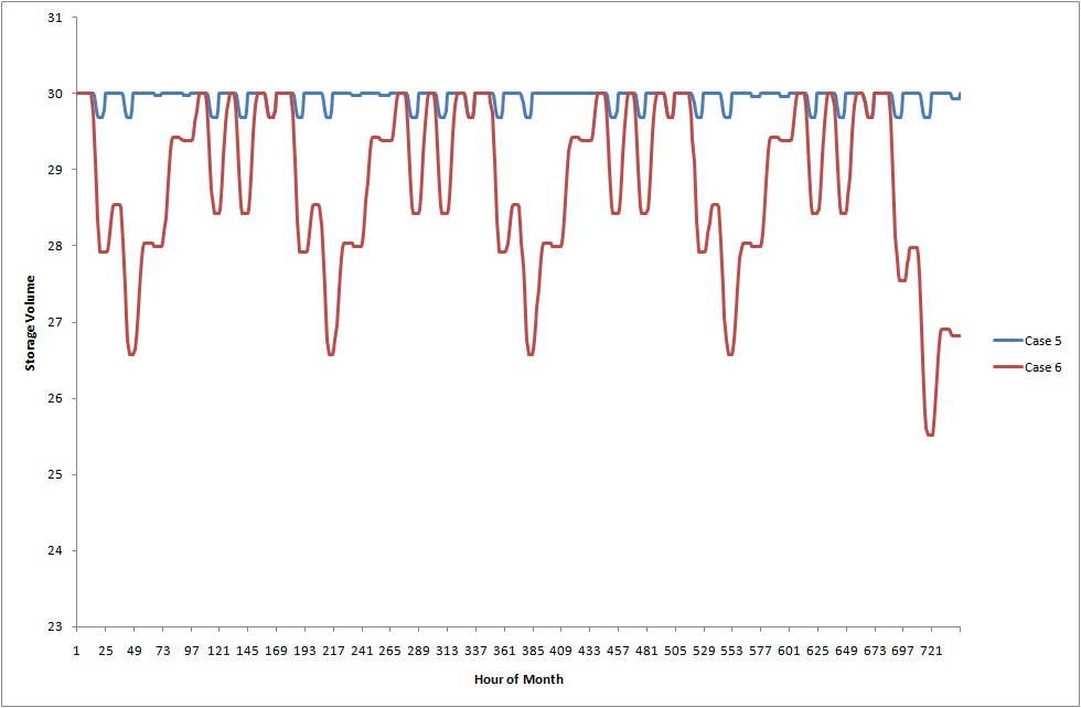 Figure
2: Pumped storage end volume (Cases 5 and 6)
Figure
2: Pumped storage end volume (Cases 5 and 6)