MT Schedule LDC Slicing Method
| Units: | - |
| Default Value: | 0 |
| Validation Rule: | In (0,1) |
| Description: | Method used to slice the LDC into blocks. |
MT Schedule LDC Slicing Method controls the approach used to slice the load duration curves into the required number of blocks, where the number of blocks is controlled by the Block Count and Last Block Count settings.
The parameter can take these values:
- Peak/Off-peak Bias (value=0)
- The slicing is done with a bias on placing blocks at the top (peak) and bottom (off-peak) of the curve, with less blocks in the middle.
- Weighted Least-squares Fit (value = 1)
- The slicing results from a least-squares fit of the step function to the duration curve where the error terms (penalties) are computed based on a weighting function.
The default weighting function is simply the original input load points, but this can be customised by defining a third-order polynomial defined by the a (constant), b (linear),c (quadratic),and d (cubic) terms. This is illustrated in the example below.
Note that points at the top (peak) and bottom (off-peak) of the duration curve may be 'pinned' and not aggregated into blocks. This is controlled by the parameters LDC Pin Top and LDC Pin Bottom. It is common for example to pin the top (peak) point so this is preserved when slicing the duration curve.
Peak/Off-peak Bias Method
Consider the load series in Figure 1, which is actual market data for South Australia in March 2011. The corresponding load duration curve is shown in Figure 2. This is simply the load values ordered highest to lowest.
Now assume that the month is to be represented by a 12-block approximation. The parameter LDC Type is "month" and Block Count is 12. Using the default method for LDC Slicing yields the 12-block duration curve shown in Figure 3. The original duration curve is shown for reference. This method automatically 'pins' the top (peak) value so in this case the first block represent the single half-hour of peak load. The remaining 11 blocks are distributed using a quadratic formula for spacing so that the block slicing is biased towards the top and bottom of the curve.
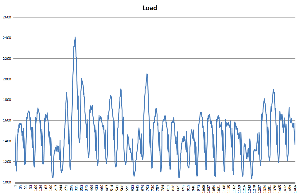 Figure 1: Load Series (1 month half-hour data)
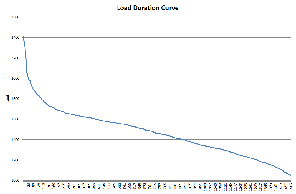 Figure 2: Load Duration Curve
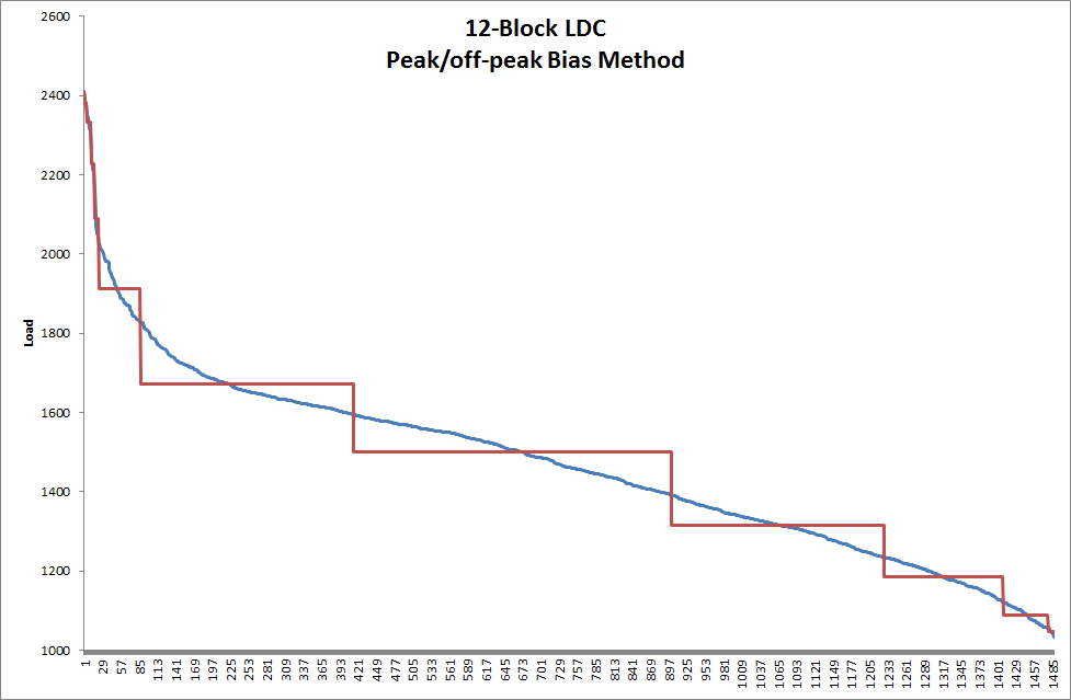 Figure 3: 12-block Load Duration Curve using Peak/off-peak Bias Method
Weighted Least-squares Fit Method
This method is a more sophisticated approach to 'fitting' the step approximation to the duration curve. The method performs an optimization that minimises the sum of squared errors i.e. the square of the difference between the original curve and the step function approximation. Further, the method allows for the definition of a weighting function that takes the place of the original curve when computing the error terms. To illustrate, consider again the duration curve in Figure 1 and the resulting 12-block approximation in Figure 3. Using the least-squares method with default weighting function yields the 12-block step function in Figure 4.
The least-squares approach has the advantage of fitting the step function more tightly to the original curve, but it does not slice the top (peak) part of the curve as closely as the peak/off-peak bias method. The purpose of the weighting function is to direct the slicing into areas of the curve that are more important and away from areas that are less important. Most commonly it is desirable to slice the duration curve with more detail in the higher load end of the curve than the lower end. To achieve this, one could perform a regression analysis of load (Q) × price (P) against the load and enter the third-order polynomial fit as the weighting function as in the following example.
Continuing the example, we will now replace the load values in the least-squares error calculation with values that better reflect the penalties for fitting errors in different parts of the curve. For example, Figure 5 shows the original load duration curve with the value of the load (Load × Price) overlaid. This value function (approximately Cost to Load) can then be regressed against load as in Figure 6 to give a third-order polynomial. In this example the polynomial is:
value(i) = = -2.6580E-05 × load(i)^3 + 1.2973E-01 × load(i)^2 - 1.4961E+02 × load(i) + 6.0826E+04These parameters are entered as:
- LDC Weight a = 6.0826E+04
- LDC Weight b = - 1.4961E+02
- LDC Weight c = 1.2973E-01
- LDC Weight d = -2.6580E-05
Entering these parameters and running the method again produces the 12-block LDC in Figure 7. The slicing changes subtly to reflect the value weighting function.
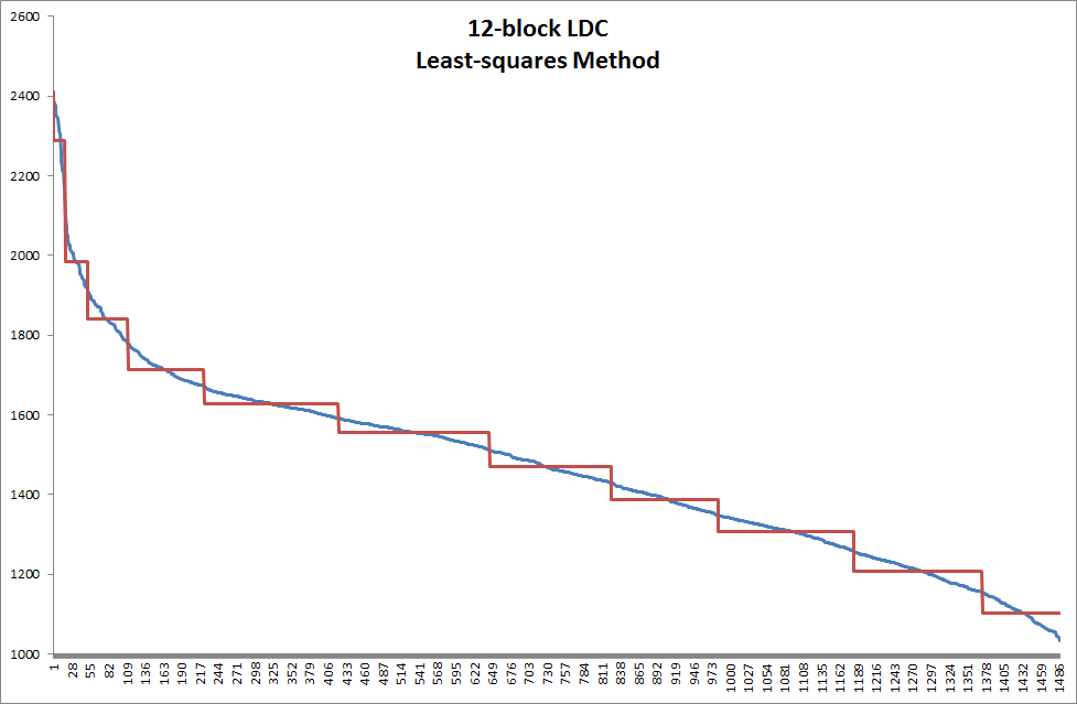 Figure 4: 12-block Load Duration Curve using Least-squares Method
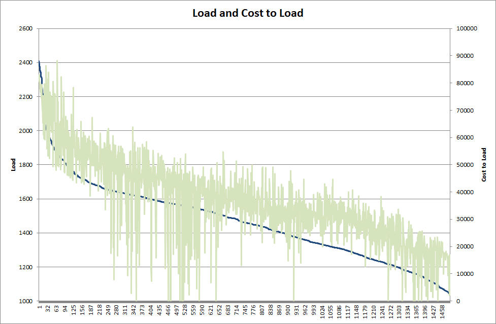 Figure 5: Load Duration Curve with Load × Price overlaid
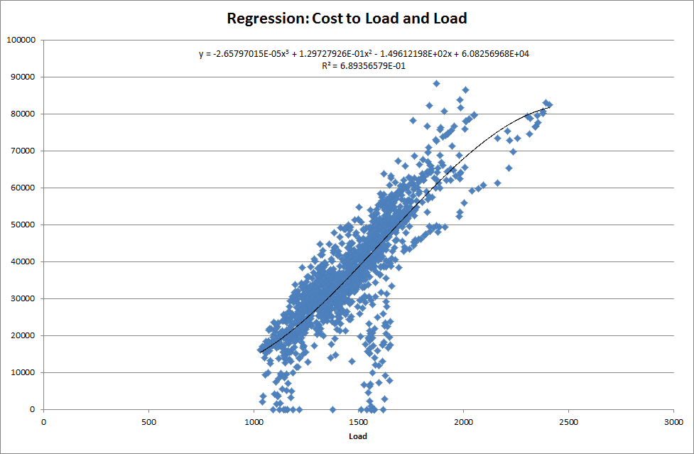 Figure 6: Regression of Load with Load × Price
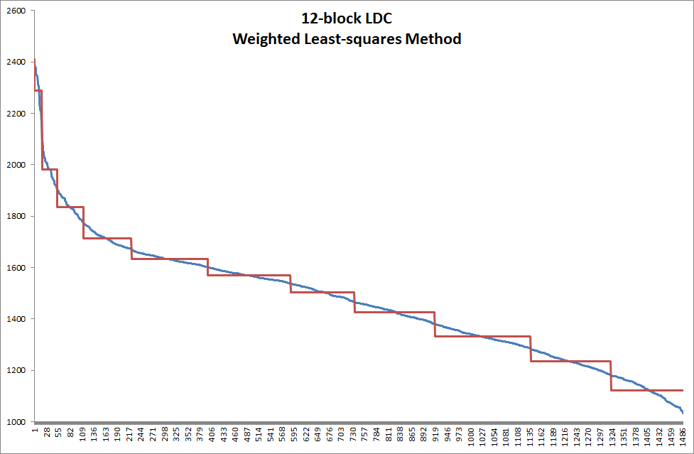 Figure 7: 12-block Load Duration Curve using Weighted Least-squares Method