Hydro-Thermal Co-ordination
Contents
1. Introduction
This section develops an example hydro-thermal coordination model as a way of demonstrating:
- A basic storage model.
- Naive versus optimized release decisions.
- Decomposition of optimal release decisions from mid to short term.
- Approximating storage modelling with energy-constrained generators
2. Formulation
The classic hydro-thermal coordination problem aims to minimise the expected value of thermal generation over some forecast horizon (T) subject to constraints on the availability of hydro generation and storage. The deterministic form of this problem can be expressed as the following optimization problem:
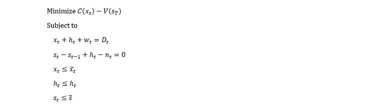
where:
Dt is the electric demand in period t
xt is the thermal generation in period t
ht is the hydro generation in period t
wt is the shortage in period t
st is the storage in period t
nt is the inflow to the storage during period t
\bar{x}_{t} is the maximum capacity of thermal generation in period t
\bar{h}_{t} is the maximum capacity of hydro generation in period t
\bar{s} is the size of the storage
C is the thermal and shortage cost function
V is the value function for storage in the final period T
3. Example System
To illustrate, assume that the thermal supply part of the cost function C is defined as in Figure 1 and that all shortage is priced at the value of lost load (a sufficiently high number) and initially that V = 0 i.e. there is no value of end-of-horizon storage. We simulate a year with demand defined with the daily profile of Figure 2 and monthly scaling factors as in Figure 3. Further, the weekend loads are scaled down by 20%. This gives the annual load duration curve of Figure 4.
For illustration, the hydro is now defined simply as:
- 1000 MW capacity
- 5000 GWh storage capacity
- 5000 GWh initial storage with no natural inflows
The hydro-thermal coordination problem is performed over the horizon T (in this example one year).
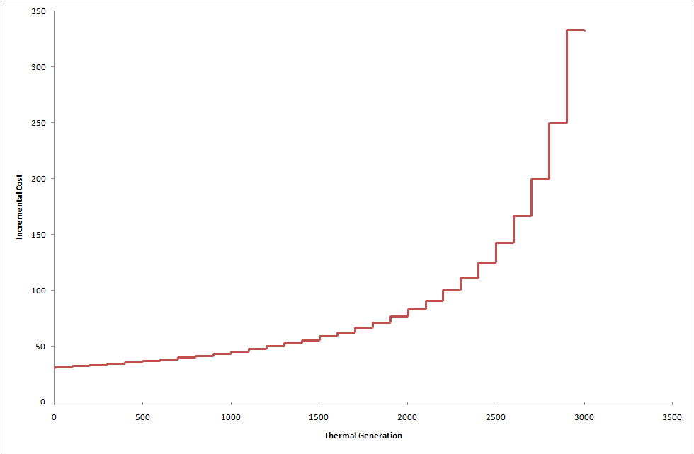 Figure 1: Thermal supply function
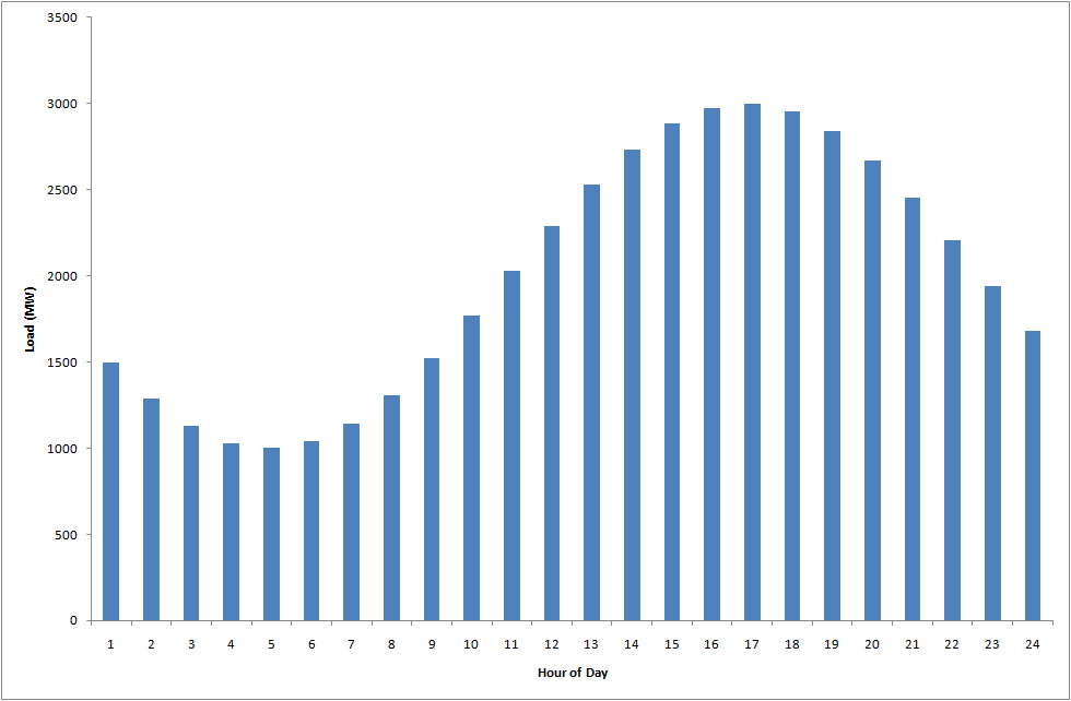 Figure 2: Load by time of day
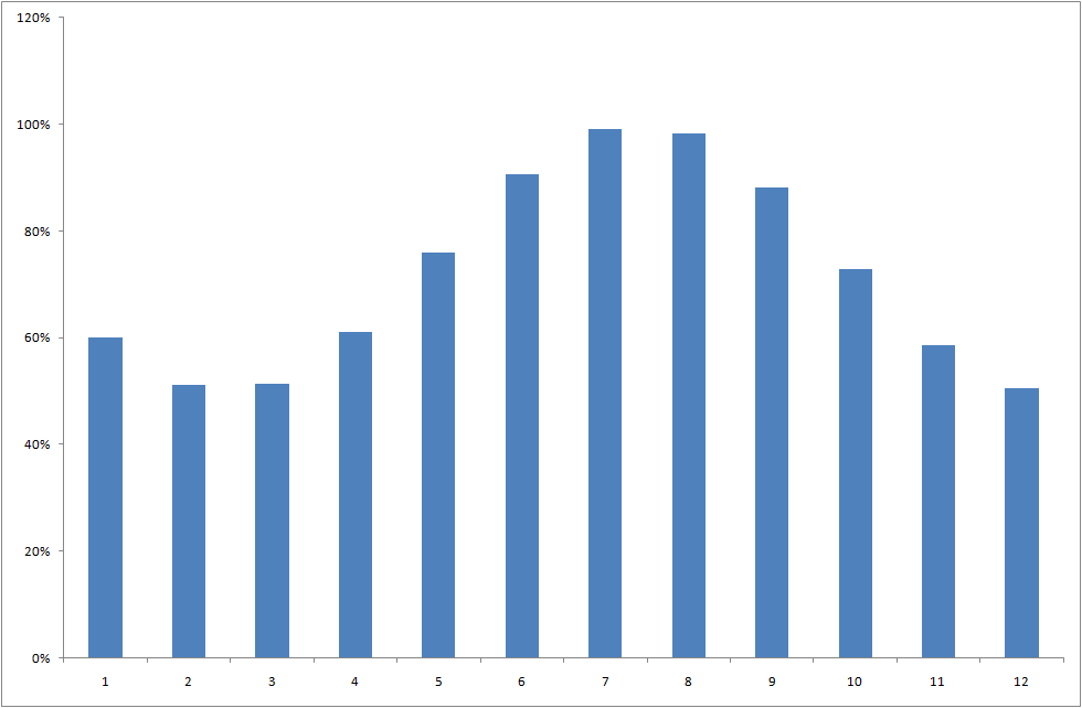 Figure 3: Load scaling factor by month of year
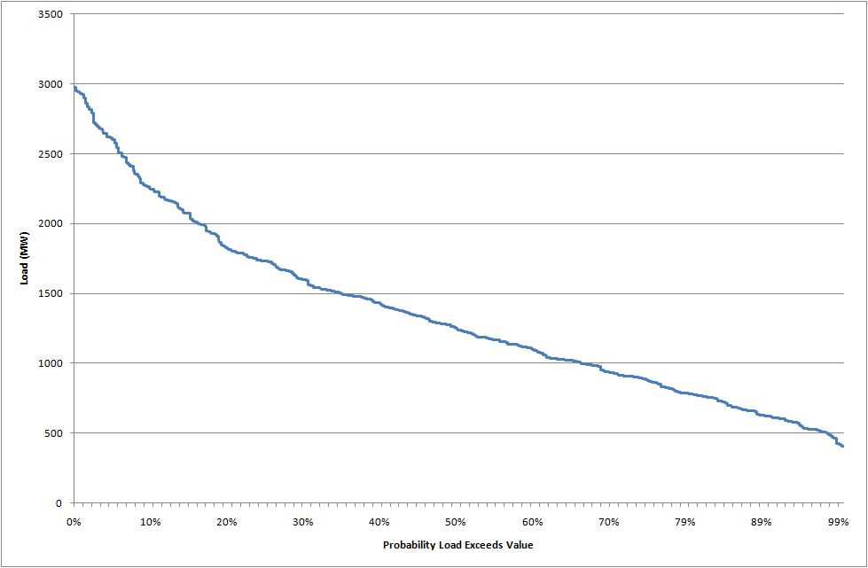 Figure 4: Load duration curve
Case 0
Thermal-only:
As a baseline, if we solve this problem with no hydro utilized, the results in Table 1 are produced. This problem can be solved independently for period t since only the hydro elements form linking constraints between periods.
Table 1: Case 0 results
| Month | Energy (GWh) | Price ($/MWh) | Generation (GWh) | Thermal Cost ($000) |
|---|---|---|---|---|
| Jan | 841 | 53 | 841 | 33330 |
| Feb | 646 | 47 | 646 | 27216 |
| Mar | 719 | 48 | 719 | 27216 |
| Apr | 830 | 54 | 830 | 33079 |
| May | 1056 | 67 | 1056 | 46132 |
| Jun | 1234 | 96 | 1234 | 61408 |
| Jul | 1397 | 141 | 1397 | 77466 |
| Aug | 1365 | 131 | 1365 | 73650 |
| Sep | 1199 | 92 | 1199 | 58194 |
| Oct | 1020 | 64 | 1020 | 43723 |
| Nov | 791 | 52 | 791 | 31030 |
| Dec | 712 | 47 | 712 | 26874 |
| Total | 11811 | 82 | 11811 | 536517 |
Case 1
Hydro-thermal solved hour-by-hour:
If we now introduce the hydro, it is clear from the hydro-thermal formulation that the optimal mix of hydro and thermal generation in any given period t is dependent on the solutions in all other periods, since the hydro is limited by the storage volume and the timing of natural inflows.
For example if we 'naively' solve this problem hour-by-hour rather than the whole T periods simultaneously, the optimal solution is to 'use up' the available hydro in each period until the resource is exhausted. The overall results are shown in Table 2, and the storage trajectory (history of end volume each hour of the year) is shown as the blue line in Figure 5 below.
This is the result that is produced when we solve the hydro-thermal coordination problem using only the ST Schedule algorithm with default settings: where the default is in fact to simulate each day independently.
Table 2: Case 1 results
| Month | Energy (GWh) | Price ($/MWh) | Generation (GWh) | Thermal Cost ($000) | Savings (Case 0 - Case 1) |
|---|---|---|---|---|---|
| Jan | 841 | 27 | 841 | 6383 | 26947 |
| Feb | 646 | 21 | 646 | 3036 | 21380 |
| Mar | 719 | 22 | 719 | 3445 | 23771 |
| Apr | 830 | 27 | 830 | 6589 | 26490 |
| May | 1056 | 34 | 1056 | 12928 | 33204 |
| Jun | 1234 | 44 | 1234 | 20685 | 40722 |
| Jul | 1397 | 51 | 1397 | 27087 | 50378 |
| Aug | 1365 | 88 | 1365 | 47738 | 25912 |
| Sep | 1199 | 92 | 1199 | 58194 | 0 |
| Oct | 1020 | 64 | 1020 | 43723 | 0 |
| Nov | 791 | 52 | 791 | 31030 | 0 |
| Dec | 712 | 47 | 712 | 26874 | 0 |
| Total | 11811 | 51 | 11811 | 287713 | 248804 |
4. Decomposition
Clearly the solution shown in Case 1 above is sub-optimal w.r.t. the original formulation. The hydro is exhausted partway through the year, and although there are significant thermal savings over Case 0, there would clearly be more savings overall if some hydro were saved for the later months of the year.
To improve on this solution we must allow the solution method to 'see' the whole simulation horizon and make the correct trade-off between using hydro 'now' versus future periods.
One approach would be to extend the step size of ST Schedule so that the entire horizon is solved in one step of size T. This might work for small problems but is impractical for real sized systems, where the number of equations required would be too large to solve.
Instead we take a two-stage approach, by enabling the MT Schedule (or LT Plan) algorithm in combination with ST Schedule. MT Schedule defaults to simulate in year-long steps, so in this case MT Schedule will find the optimal hydro release policy. By default MT Schedule uses a reduced chronology, rather than simulating every interval, thus if we wish to simulate to full resolution we must also run ST Schedule.
The two (or more) simulation 'phases' are automatically linked together, running MT Schedule first (and/or LT Plan), then ST Schedule but with the ST Schedule hydro release policy guided by solutions of the preceding phase.
In effect long or mid-term phase decomposes the hydro-thermal coordination problem into a number of sub-problems that are then solved by ST Schedule. This multiple-stage approach allows for the efficient solution of very large systems down to full chronological detail.
Case 2
Two-stage optimization with MT Schedule and ST Schedule:
The results for this case are shown in Table 3, and the optimal storage trajectory is the red line.
Table 3: Case 2 results
| Month | Energy (GWh) | Price ($/MWh) | Generation (GWh) | Thermal Cost ($000) | Savings (Case 0 - Case 2) |
|---|---|---|---|---|---|
| Jan | 841 | 39 | 841 | 16667 | 16664 |
| Feb | 646 | 38 | 646 | 14275 | 10141 |
| Mar | 719 | 38 | 719 | 15833 | 11382 |
| Apr | 830 | 39 | 830 | 16257 | 16822 |
| May | 1056 | 42 | 1056 | 20463 | 25670 |
| Jun | 1234 | 48 | 1234 | 26080 | 35328 |
| Jul | 1397 | 53 | 1397 | 31832 | 45634 |
| Aug | 1365 | 52 | 1365 | 30727 | 42923 |
| Sep | 1199 | 47 | 1199 | 24956 | 33238 |
| Oct | 1020 | 41 | 1020 | 19685 | 24038 |
| Nov | 791 | 39 | 791 | 15960 | 15070 |
| Dec | 712 | 38 | 712 | 15803 | 11071 |
| Total | 11811 | 44 | 11811 | 248537 | 287980 |
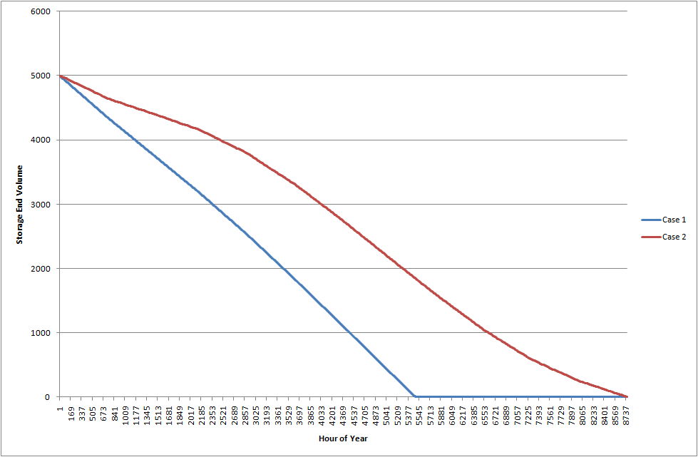 Figure 5: Storage trajectories (Cases 1 and 2)
5. Natural Inflows
Thus far we have ignored two elements of the hydro-thermal coordination problem: natural inflows, and the value of end-period storage. To illustrate, assume now that inflows to the storage occur in the monthly pattern shown in Table 4 and illustrated in Figure 6; and that the storage starts the year at 75% full and must return to that level at the end of the year.
These are typical assumptions for modelling storages that 'cycle' over a year or less. In reality some storages have multi-annual cycles, and these can be handled either by decomposing with LT Plan which defaults to multi-annual optimization or by extending the optimization step of MT Schedule.
We define the natural inflow as a dynamic property Storage Natural Inflow. The values are rates, not aggregate quantities, thus we must convert the monthly totals in the "Total (GWh)" column of Table 4 to the equivalent inflow rates in shown in the "Rate (MW)" column.
Defining Storage Natural Inflow automatically invokes the "recycle" method for end storage valuation, meaning that MT Schedule will impose the constraint:
sT=s0
This behaviour can be overridden as shown in see the End Effects Method topic.
Table 4: Natural inflows
| Month | Proportion | Total (GWh) | Hours | Rate (MW) |
|---|---|---|---|---|
| Jan | 0.04 | 200 | 744 | 268.82 |
| Feb | 0.02 | 100 | 672 | 148.81 |
| Mar | 0.03 | 150 | 744 | 201.61 |
| Apr | 0.05 | 250 | 720 | 347.22 |
| May | 0.07 | 350 | 744 | 470.43 |
| Jun | 0.08 | 400 | 720 | 555.56 |
| Jul | 0.1 | 500 | 744 | 1008.06 |
| Aug | 0.15 | 750 | 744 | 1008.06 |
| Sep | 0.18 | 900 | 720 | 625 |
| Oct | 0.13 | 650 | 744 | 873.66 |
| Nov | 0.09 | 450 | 720 | 625 |
| Dec | 0.06 | 300 | 744 | 403.23 |
| Total | 1 | 5000 | 8760 | 570.78 |
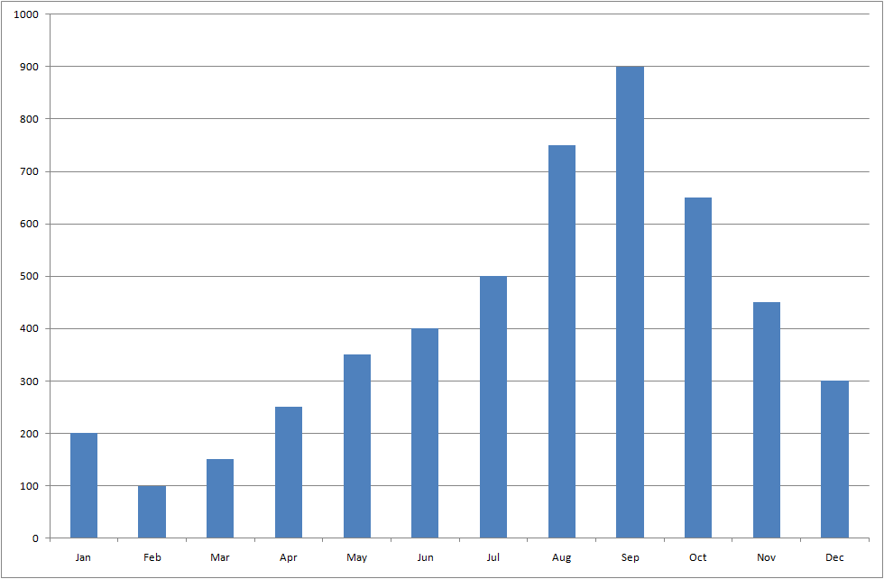 Figure 6: Natural inflows by month
Case 3
Natural inflows and recycled storage:
The solution to this case is shown in Table 5. The storage monthly inflows, releases, and end volume is illustrated in Figure 7. Note that the thermal cost in this case is very close to Case 2 indicating that the two-stage optimization has efficiently optimized the use of the storage in order to compensate for the fact that most of the inflows arrive after the peak demand time.
NOTE: This level of optimization might not be achievable in reality because of uncertainty in the flow forecast, and this is discussed in the article, Hydro Reservoirs.
Table 5: Case 3 results
| Month | Energy | Price | Generation | Thermal Cost | Savings (Case 0 - Case 3) |
|---|---|---|---|---|---|
| Jan | 841 | 39 | 841 | 16843 | 16487 |
| Feb | 646 | 38 | 646 | 14413 | 10004 |
| Mar | 719 | 38 | 719 | 15662 | 11554 |
| Apr | 830 | 39 | 830 | 16172 | 16907 |
| May | 1056 | 42 | 1056 | 20627 | 25505 |
| Jun | 1234 | 48 | 1234 | 26946 | 35362 |
| Jul | 1397 | 53 | 1397 | 31824 | 45641 |
| Aug | 1365 | 52 | 1365 | 30681 | 42968 |
| Sep | 1199 | 47 | 1199 | 24711 | 33483 |
| Oct | 1020 | 41 | 1020 | 19731 | 23992 |
| Nov | 791 | 39 | 791 | 15940 | 15090 |
| Dec | 712 | 38 | 712 | 15917 | 10975 |
| Total | 11811 | 44 | 11811 | 248567 | 287950 |
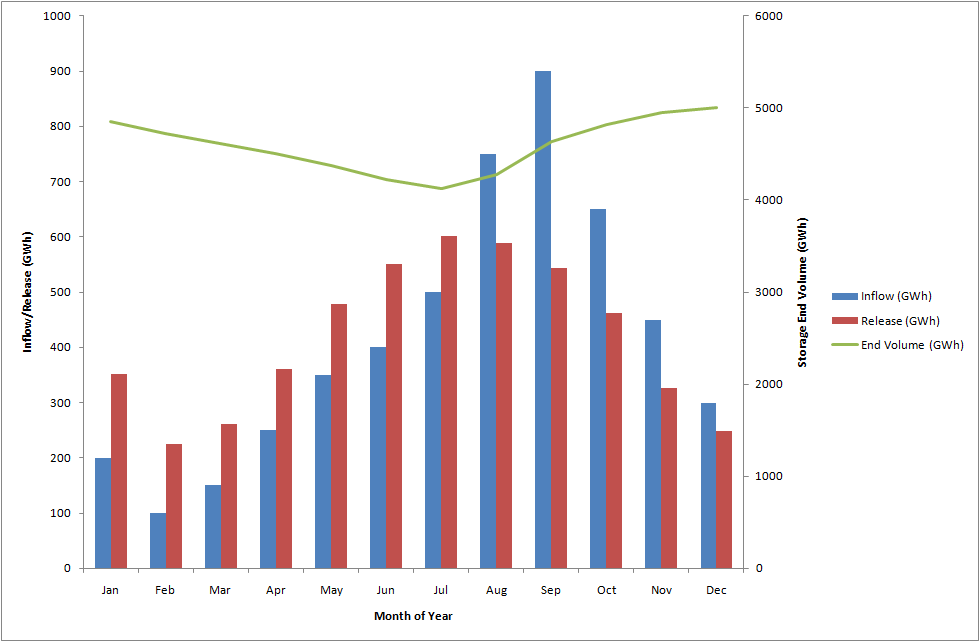 Figure 7: Case 3 storage inflow, release and volume by month
6. Energy-constrained Generator
Assuming the hydro systems in our simulation are only as complex as this example or that the available data does not permit the modelling of storages even in this detail we can approximate the hydro system as an energy-constrained generator. This means modelling the hydro using only a Generator object, but adding properties that define:
- Limits on the total generation available each (for example) month; and
- Minimum generation reflective of the need to generate at times of high inflows in order to avoid spill.
To illustrate, consider the solution to Case 3 above. This solution can be approximated using a Generator with monthly energy limits and minimum hourly generation as in Table 6.
Table 6: Monthly energy limits and minimum load
| Month | Energy(GWh) | Min Load (MW) |
|---|---|---|
| Jan | 351.03 | 0 |
| Feb | 277.89 | 0 |
| Mar | 252.94 | 0 |
| Apr | 354.97 | 0 |
| May | 478.96 | 0 |
| Jun | 558.75 | 134.98 |
| Jul | 605.29 | 191.95 |
| Aug | 600.84 | 199.71 |
| Sep | 538.47 | 81.53 |
| Oct | 463.72 | 0 |
| Nov | 326.74 | 0 |
| Dec | 240.4 | 0 |
| Total | 5000 |
These data are entered as Generator Max Energy Month and Min Load with the Timeslice field set "M1", "M2", ..., "M12". Note how Min Load is a rate, whereas the energy limit is a quantity.
Similar to Case 3 you must enable MT Schedule so that these monthly energy constraints can be decomposed into limits that ST Schedule can follow.
Case 4
Approximation using an energy-constrained generator:
The results for this case are in Table 7. Figure 8 illustrates the generation duration curve for the hydro generator in these two cases: remembering that Case 3 models the hydro with an attached storage and natural inflows, whereas Case 4 models it is a 'simple' energy-constrained generator. These results illustrate how a hydro with storage can be nicely approximated as an energy-constrained generator with energy limits and minimum generation constraints.
In the next section we expand on this example, introducing complexities that cannot be handled using this approximate method and that must be modelled using the more advanced features of the hydro model.
Table 7: Case 4 results
| Month | Energy | Price | Generation | Thermal Cost | Savings (Case 0 - Case 4) |
|---|---|---|---|---|---|
| Jan | 841 | 39 | 841 | 16887 | 16443 |
| Feb | 646 | 38 | 646 | 14321 | 10095 |
| Mar | 719 | 38 | 719 | 15978 | 11238 |
| Apr | 830 | 39 | 830 | 16361 | 16718 |
| May | 1056 | 42 | 1056 | 20620 | 25513 |
| Jun | 1234 | 48 | 1234 | 25752 | 35656 |
| Jul | 1397 | 53 | 1397 | 31701 | 45764 |
| Aug | 1365 | 52 | 1365 | 30224 | 43426 |
| Sep | 1199 | 47 | 1199 | 24886 | 33308 |
| Oct | 1020 | 41 | 1020 | 10689 | 24033 |
| Nov | 791 | 39 | 791 | 15934 | 15096 |
| Dec | 712 | 38 | 712 | 16190 | 10684 |
| Total | 11811 | 44 | 11811 | 248543 | 287974 |
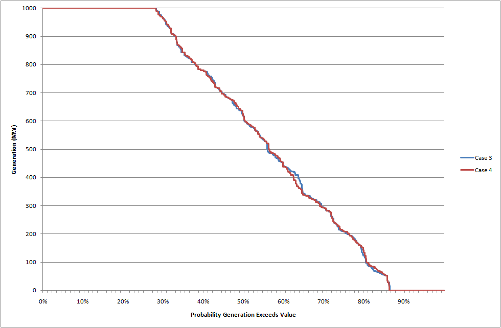 Figure 8: Generation duration curves (Cases 3 and 4)