Map Visualization
Contents
1. Input Map Layout
1.1. Access to the Visualization Window
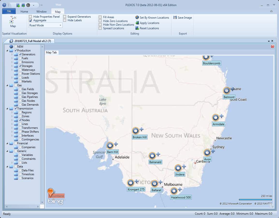
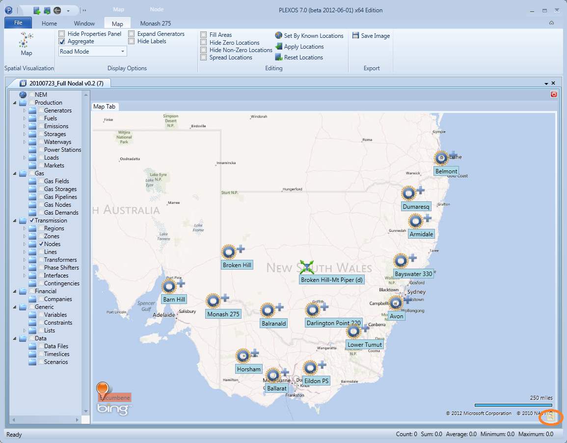
The visualization window is accessed using the Map button from the Map tab of ribbon-style menu.
Map visualization utilises latitude and longitude coordinates as a part of the application. If you wish to avail of this, ensure to enable the coordinates of objects in the Config screen under Attributes for each object.
Spatial visualization uses the Microsoft Bing Map to locate and display objects. The application requires an internet connection to access the Bing map and online spatial services. The feature establishes access to the Bing website and opens the visualization window only if a connection is made.
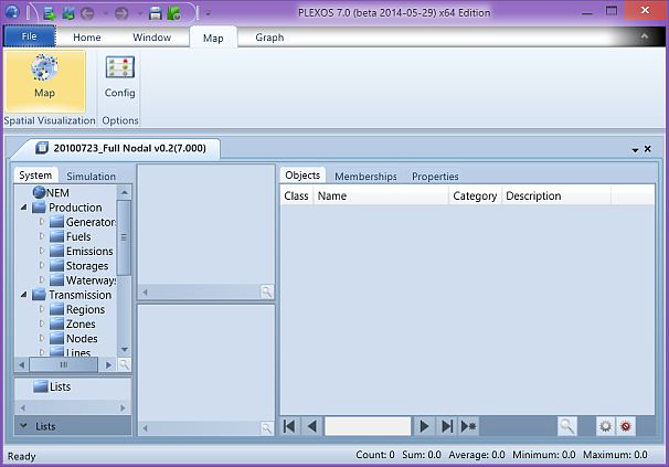
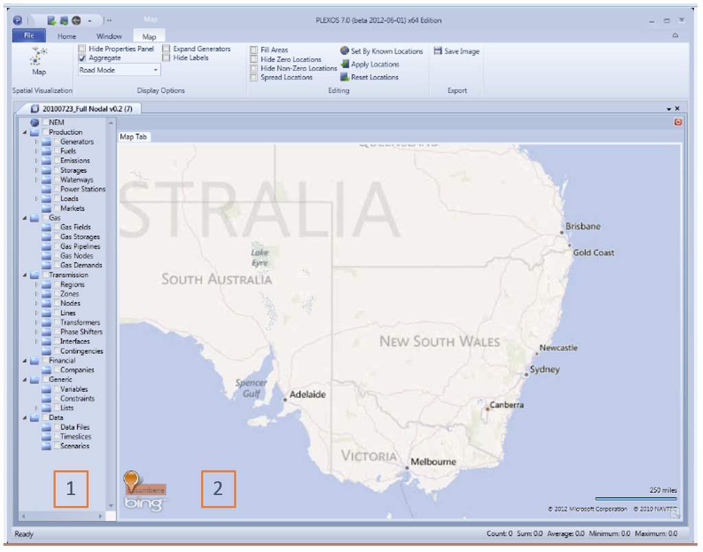
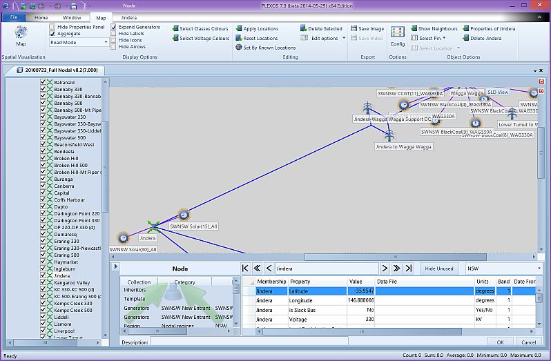
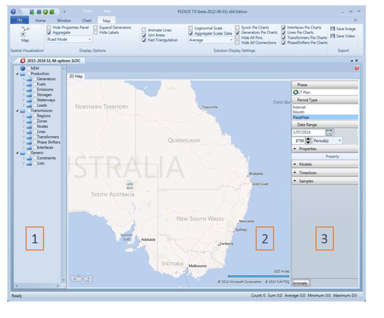
1.2. Visualization Window Layout
The visualization window has two areas;
- Tree of filters: It is organised like the tree of objects in the main application
- Map: Displays the map of visualized objects
Most controls are located on the map tab of the ribbon style menu.
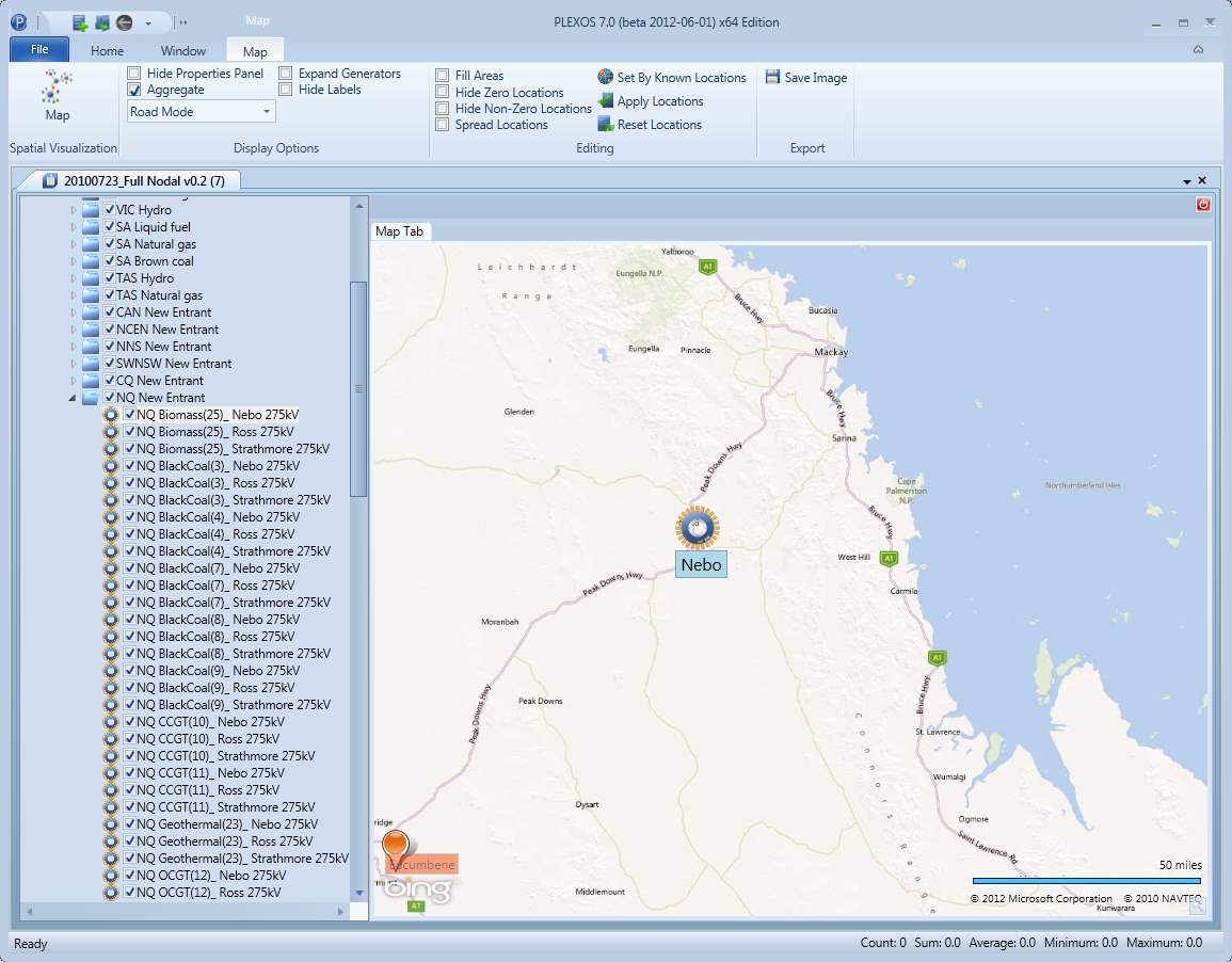
1.3. Tree of Filters
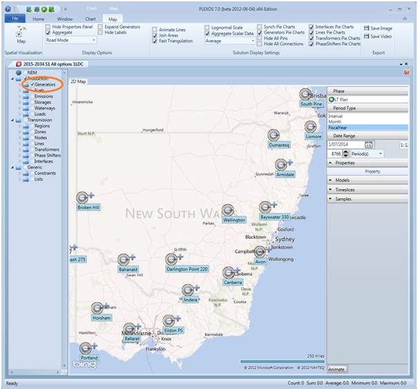
Objects can be put to or removed from the map by checking or unchecking corresponding filters. Enabling a filter makes all objects associated via memberships also visible, the corresponding nodes on the tree are also checked. For example: when we enable the Generators filter on the tree, this will enable all the nodes and storages that represent these generators (icons of generators with the node names under them).
Disabling the Generators filter will uncheck all the filters and remove objects from the map.
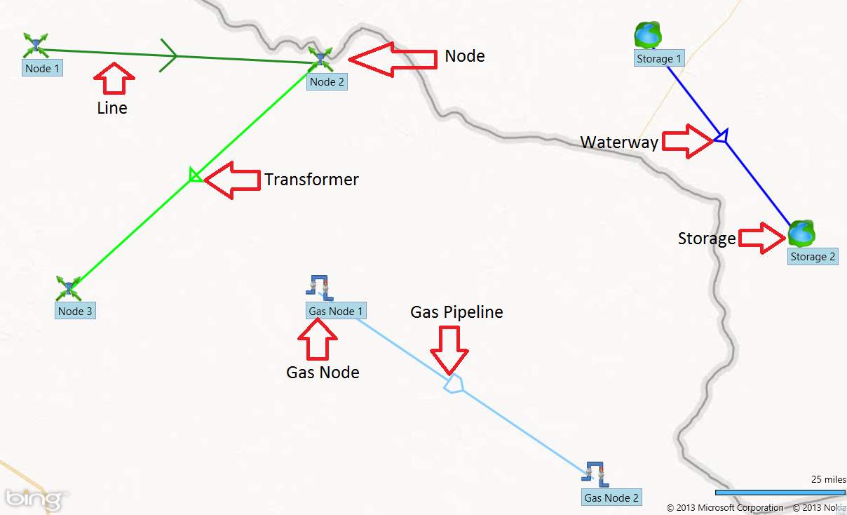
NOTE: Currently only nodes, generators, storages, gas nodes, gas storages, water nodes, water storages, companies, loads, power stations, gas fields, gas demands, water demands, lines, transformers, gas pipelines, water pipeline and waterways can be visualized.
When a particular node is selected, it's icon on the map becomes larger (if a line or waterway is selected then it becomes red). Moving or zooming the map returns items to their normal state. Double-click on a tree node centres the map about that object (provided that the object is checked and has non-zero coordinates). The right click menu options on an object are to highlight that object (same action as double-click) or delete it.
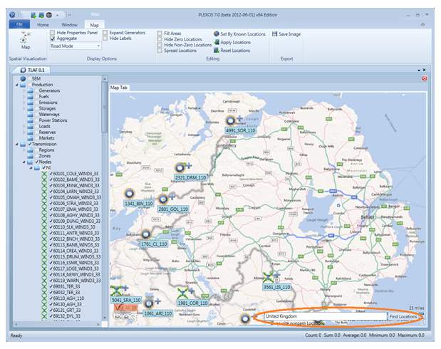
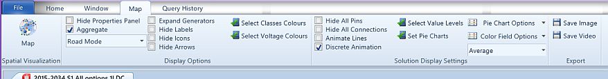
1.4. Map Controls
Positioning of the map is done via a left click of the mouse, hold and drag to the required position. Zoom in or out by rolling the mouse wheel or use the + and - keys on the keyboard. The map has four groups of controls:
Spatial Visualization
Map: Turns on the map application.
Display Options Group
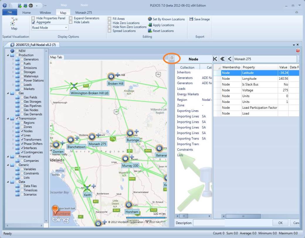
Hide Properties Panel: Hides/ displays the property pane for selected element at the bottom or right of the map. The property pane can also be shown if user double-clicks an object on the map.
Aggregate: Toggles between displaying individual nodes or an aggregated node to represent nearby nodes. May help in simplifying a busy map.
Expand Generators: Arrange generators associated with a node around that node (when the number of associated generators is less than 20).
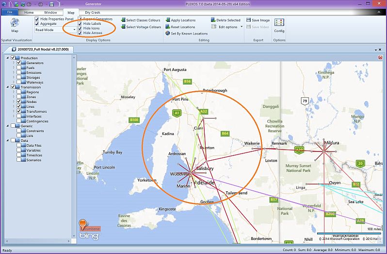
Hide Labels: Hides/ Displays the label of each object name. This can be useful to de-clutter a map or display a generic over view of the infrastructure in an area.
Hide Icons: Option collapses pins icons to small grey dots, regular icon appears when mouse pointer hovers over the pin and collapses back when mouse leaves that pin.
Hide Arrows: "Option removes arrows from all of the lines.
Map Mode: User can select from "Road Mode" (default), "Aerial Mode, "Faded Road Mode" - map titles become faded to make PLEXOS objects look more distinct and "Merkator Mode" -grey titles with no topographic objects.
Select Classes Colours: User can select colour for each transportation class of objects (Line, Transformer, Waterway, Gas Pipeline or Water Pipeline). This selection is saved and applies to all visualization layouts.
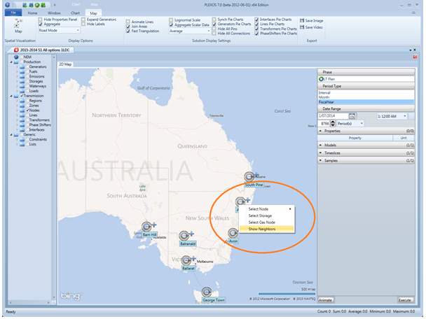
Select Voltage Colours: User can select colour for each value of voltage of lines and transformers. Also, user can select level of significant voltage ("High Voltage"), so that lines and transformers with voltage equal or above that level will have thicker lines. This selection is saved and applies to all visualization layouts.
While the above image is default view, pressing the right arrow (circled in orange above) moves the property pane to the right edge of the window.
Aggregate:
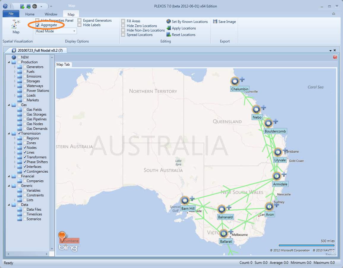
Aggregate on
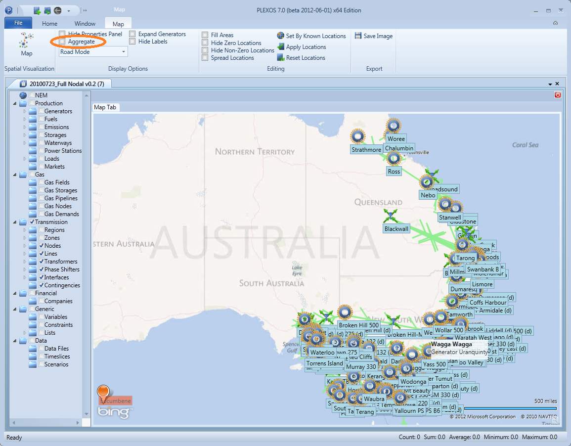
Aggregate off
Expand Generators: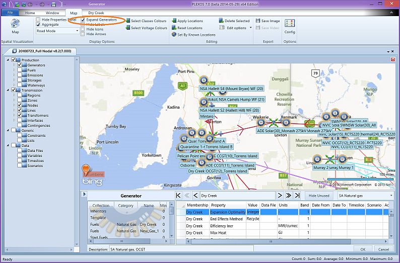
Hide Labels:
Map mode selection:
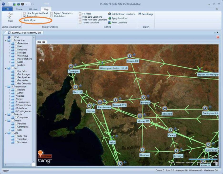
Aerial Mode
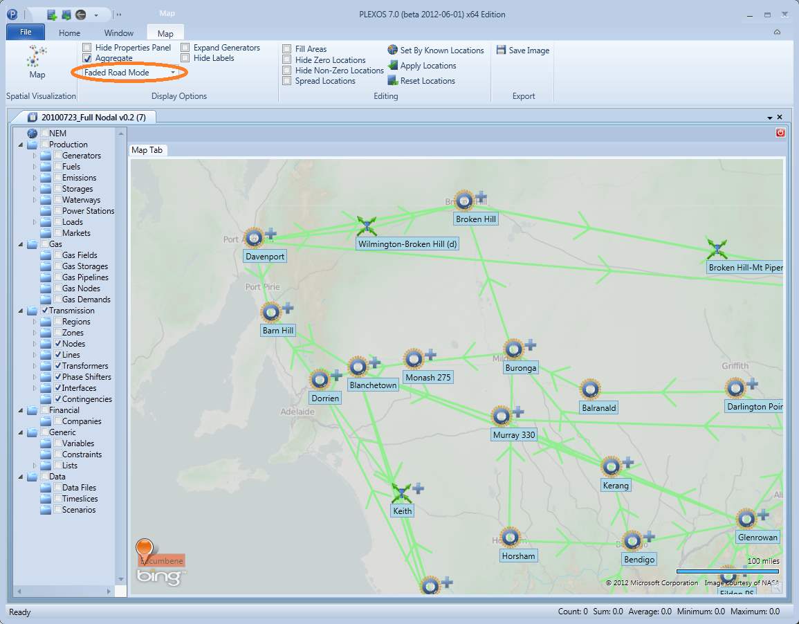
Faded Road Mode
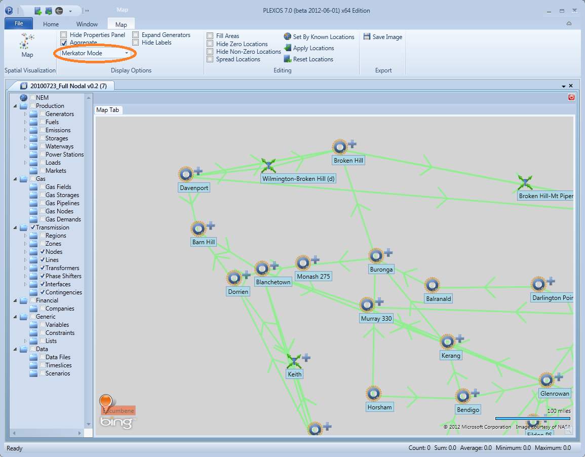
Merkator Mode
Transportation objects colours selection: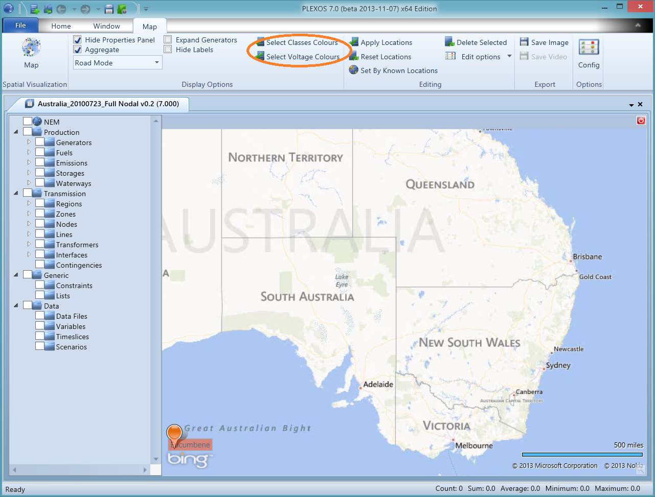
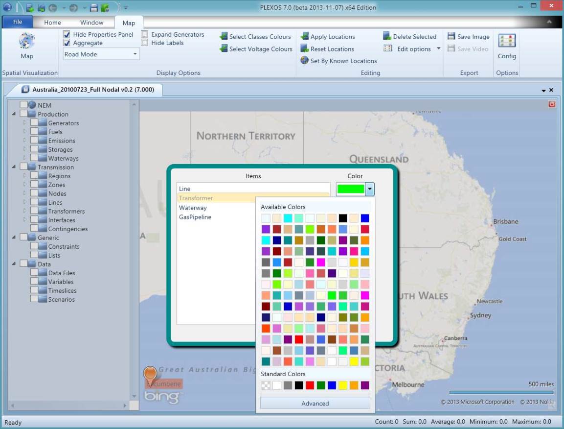
Colours selection for classes
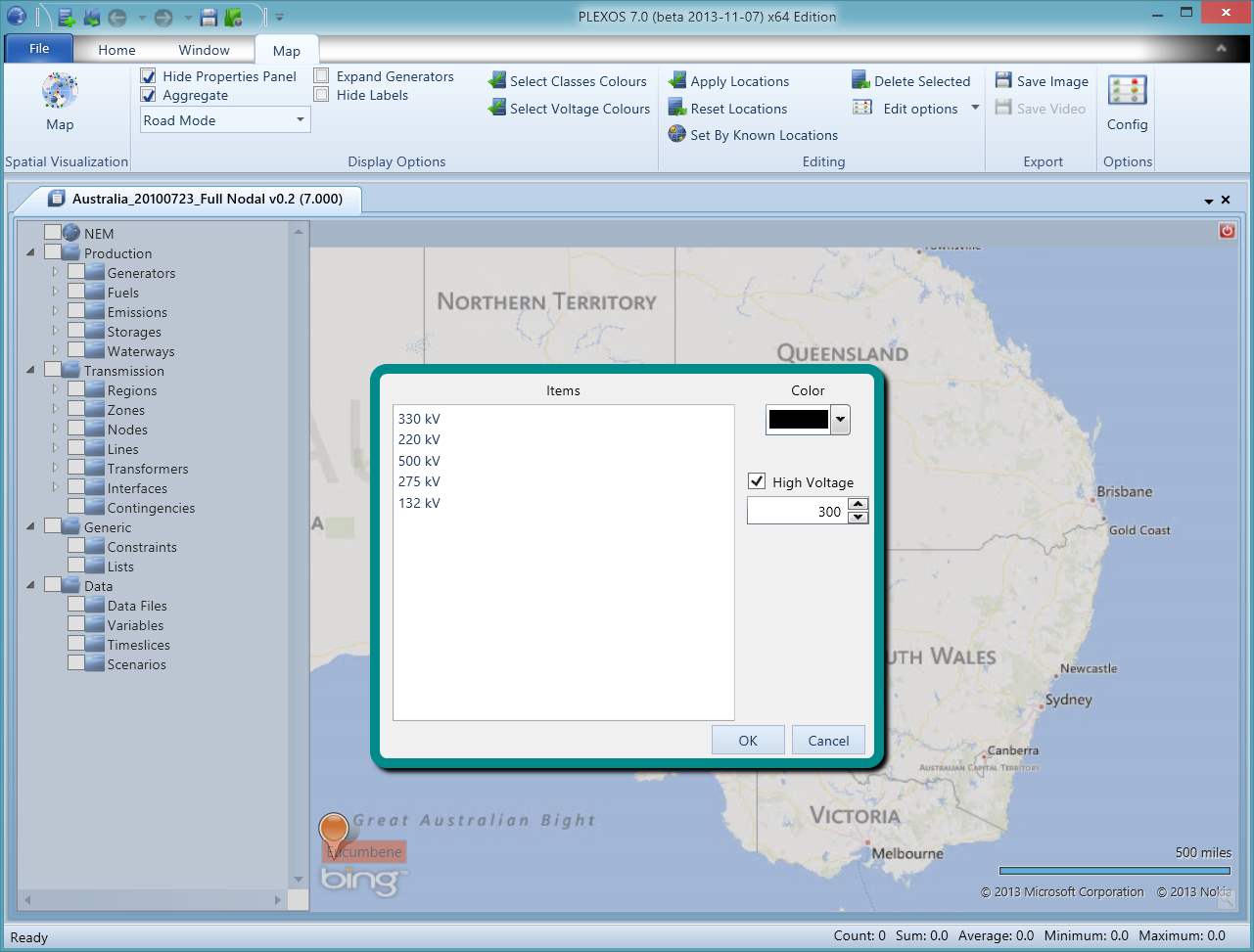
Colours selection for voltages, and setting a level of significant voltage
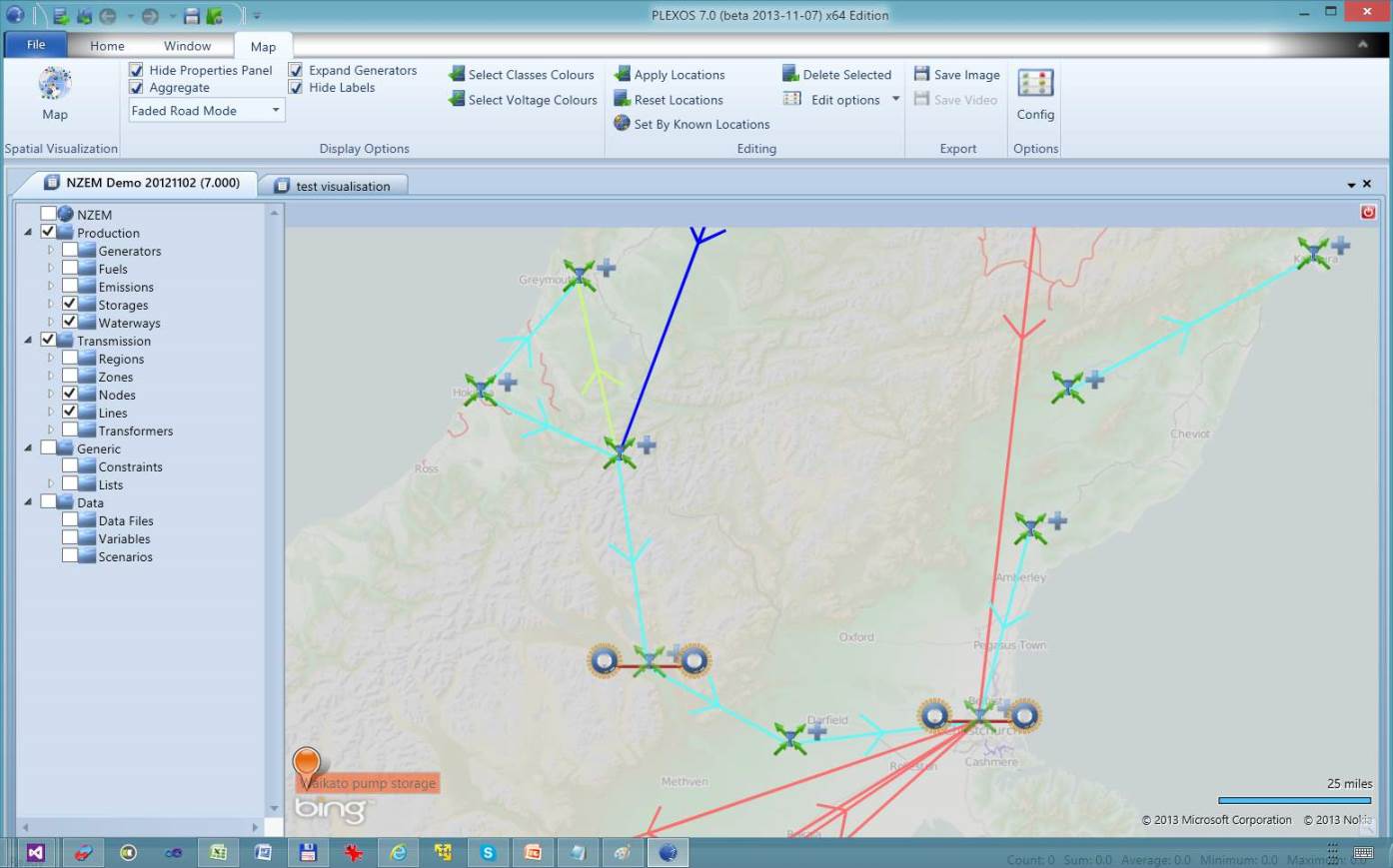
Coloured transportation network
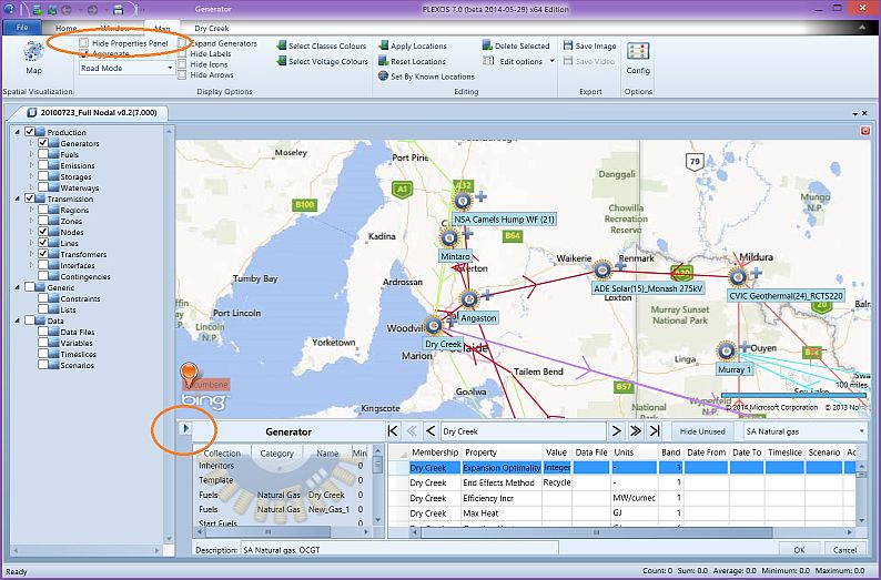
Editing Group
The group is only visible when a visualized model has objects with zero longitude and zero latitude (considered as not localised objects or zero location objects) or objects being edited. It consists of:
Fill Areas: Filling inner areas of zones and regions.
Set Nodes by Known Locations: Function locates not localised PLEXOS objects according to their connections (via lines or waterways) to PLEXOS objects with known locations. Described in the Automated Positioning section of the manual.
Apply Locations: Applies all the changes made to objects being edited.
Reset Locations: Clears all the changes made to the objects Bing edited.
Hide non Zero Locations: Hides all objects with non-zero locations on the map (without changing states of filters).
Spread Locations: Spreads locations of all PLEXOS objects which got exact same location after automatic positioning. Described in the automated positioning section of the manual.
Delete Selected: Deletes all selected pin items from database.
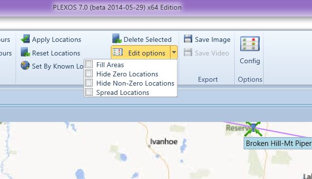
Expanded editing options
Export Group
Save Image: Saves current map view as png image file.
The pushpin icon in the lower left corner of the map represents PLEXOS objects with zero location - Described in the Manual Positioning section of the manual. Lower right corner group's visibility depends on search Mode toggle button (see the looking glass icon) in the very lower right corner of visualization window.
Lookup controls toggle
Pressing the toggle button once opens filter free search controls (very similar to ones used in PLEXOS GUI), which is used to find filter tree on the right pert of visualization window, works the same way such search works ins the rest of the GUI.

Pressing the toggle a second time hides the tree search controls and opens the location search controls group.
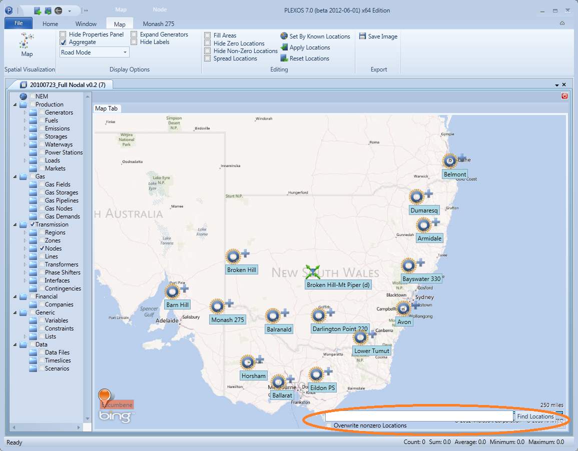
Pressing the toggle a third time hides the controls.
1.5. Map Objects
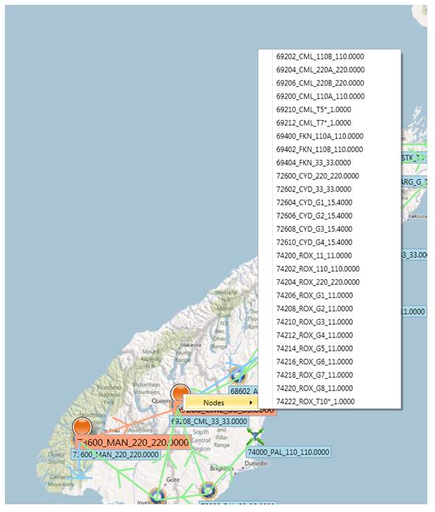
Double-click on a pin object, the property window of the underlying PLEXOS object will open. The right-click menu of pin objects (nodes, gas nodes, water nodes, generators, storages, gas storages and water storages) contains six options.
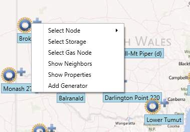
Selecting an item from any of the lists sets the underlying objects as the aggregation centre.
Select Node: Contains list of nodes aggregated by the pin object.
Select Storage: Contains the list of storages aggregated by the pin object.
Select Gas Node: Contains list of gas nodes aggregated by the pin object.
Select Water Node: Contains list of water nodes aggregated by the pin object.
Show Neighbours: Opens a new window on top of the map displaying all the direct memberships of the chosen pin object.
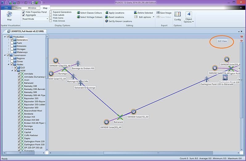
Neighbour view visualization feature is available for Nodes, Gas Nodes and Water Nodes from all of the visual layout types (Input/Output, Map/Mapless(Graph)) and also it has an option of SLD style presentation (SLD is the only type of Neighbour view available for Graph layouts) or PLEXOS style (graph style similar to graph visualisation). The function is designed for electrical and gas transmission and is available from pins right-click menu (Node, Gas Node or Water Node pins in case of Graph layouts). Once opened the view represents transmissions object connected to a selected node in a Single Line Diagram style, using PLEXOS icons for object's type indication (All but Nodes, which are presented as Once opened the view represents transmissions object connected to a selected node in a Single Line Diagram style, using PLEXOS icons for object's type indication (All but Nodes, which are presented as thick bar elements).
Neighbours of the Balranald node in SLD style.
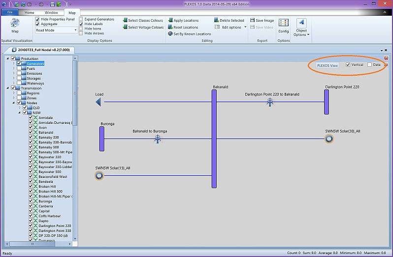
Neighbours of the Balranald node PLEXOS style.
For the sake of performance all data reporting (Voltage, Rating, Max Capacity, etc.) is turned off by default, but can be switched on by clicking Data checkbox.
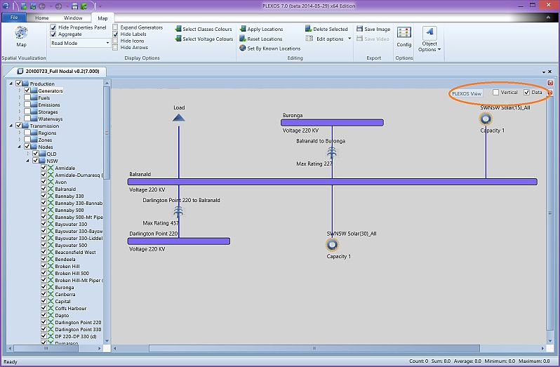
Horizontal layout and data display is on.
From the right-click menu user can open properties for an object, navigate to next or get back to that object on map layout.
Exit button to leave Map Visualization mode.
Show Properties: Opens the property pane for a PLEXOS object associated with the chosen pin.
Right-click menu of lines, gas pipelines, transformers and waterways
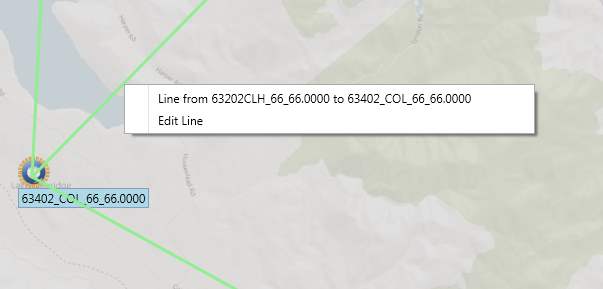
Menu consists of the names of lines and waterways followed by Edit Line menu item. Selecting line or waterway name will open property window of the underlying PLEXOS object. Selecting Edit Line will put the line into edit mode, described in the manual positioning section of the manual.
1.6. Manual Positioning
New nodes and storages can be added via a right-click on the point of the map with the desired location.
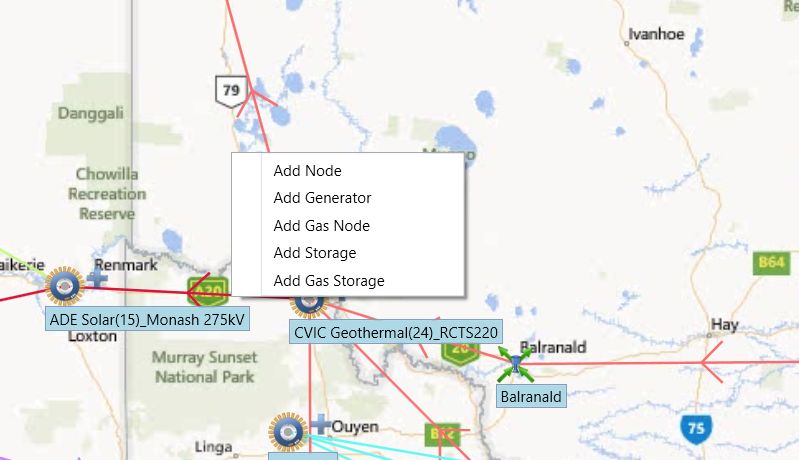
Choosing to add a new object from this menu open the new object dialogue, where the user can create an object name, description and select a category.
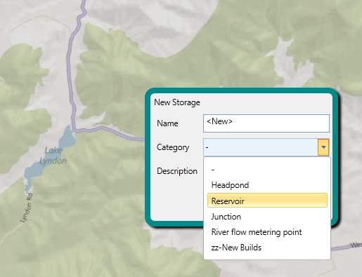
Creating up new object
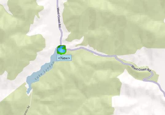
New storage created
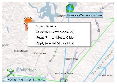
In order to move any pin object manually, hold the control key and drag the pin with a left click to the desired location. Both pins can be manually positioned, those which are already positioned and put on the map (pin icon will change to standard Bing Map push pin icon in this case) and those with zero locations (from the lower left part of the map area). Once the objects are placed the user can either apply or reset the changes by clicking the Apply Locations or Reset Locations buttons (for bulk apply or reset) or select the corresponding menu items from the right-click menu or hold A or R key and click the pin for Apply or Reset respectively. User also can clear objects location (set to zero) by pressing and holding Z-key and right-clicking modified object.
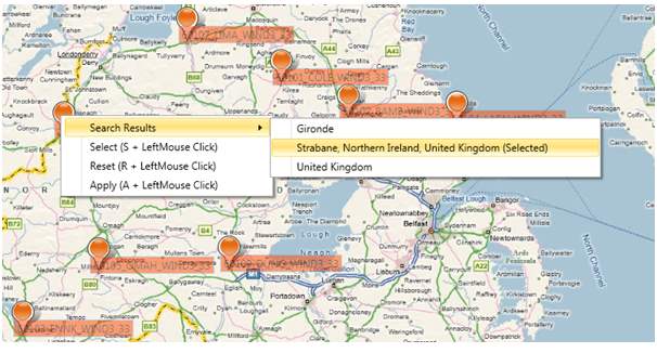
Menu Items "Search Results" and Select are discussed in the Automated Positioning section of the manual.
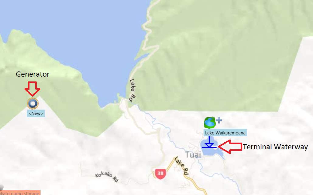
Transport type objects can be created by pressing and holding L key and clicking on pins. The type of object will be selected according to the type of pin clicked:
- Line or Transformer for nodes. The default is line, in order to create a transformer, select any transformer or transformers class group from the filters tree.
- Waterway for storages.
- Gas Pipeline for gas nodes
- Water Pipeline for water nodes.
The first pin clicked will form the From membership with the newly created object and the second pin will form the To membership. You will know the pin object is selected when a Bing Map icon appears over the selected object.
After the second or To pin is selected the transport object is displayed in orange indicating edit mode and a new object dialogue will open. Input name, description and select lines, gas pipelines, water pipelines or waterways category. If the L key is released before the To object is selected, the line (or pipeline or Transformer) will automatically be deleted as the essential memberships were not created. This is not the case if a Waterway object is created as a terminal waterway needs only a From membership.
If the Name field is left blank, PLEXOS creates an automatic name in the form of memberships, for example if a newly created line is going From Node 1 To Node 2 then the line will be named Node 1 to Node 2.
The user can select which particular node or storage he wants for each of the ends using the right click menu and either:
- Work through the property pane by selecting the object name.
- Select Edit Line, hold control and drag the appropriate pin icons onto the required node or storage object.
After all the manipulations have been made, the line can be applied by clicking the Apply Locations or Reset Locations button.
Gas pipeline, Water pipeline, Line or waterway can be put into edit mode using Edit Line option from right-click menu. In edit mode user can change nodes or storages, or delete line by removing its ends (user has to click on each of them).
1.7. Automated Positioning
In order to make positioning of objects easier, the visualization window implements several ways of automatic object positioning. Possible location of object (node or storage) can be found using the online Bing spatial services by object name, description, user input keywords or category information. In order to use this type of search, select an object or class of objects in filter tree node. Press the looking glass toggle twice (bottom right corner) to open the Location search controls group. Type the a keyword in the search text box if needed, check "Overwrite nonzero Locations" if the search is to locate objects that already have non-zero longitudes and latitudes, uncheck otherwise.
Note: If a user would like to make use of this functionality, geographical information needs to be entered in either the object name or description when an object is created.
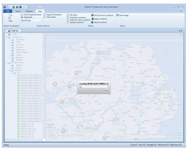
Press Find Locations. You will see progress dialogue with a progress bar and stop button to interrupt search.
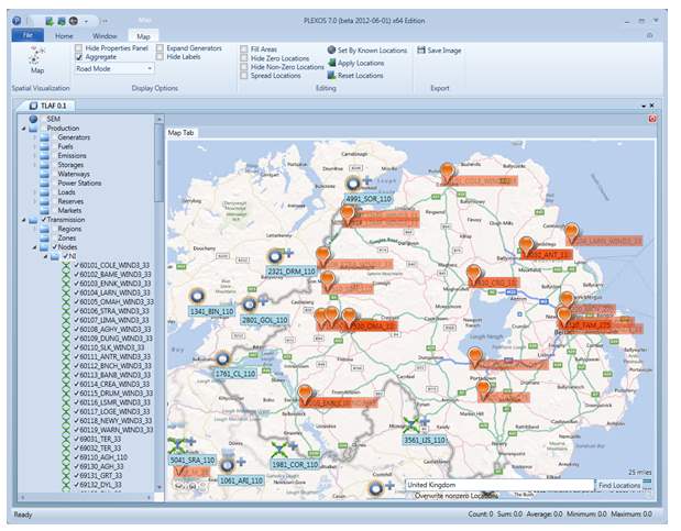
After the search is complete, nodes with at least one location within the map's field of view are put on the map in edit mode, where the user can select a more appropriate location from the list of found locations for the node (in right-click menu) or select the node (from the same menu) and rerun the search for this particular object if needed.
Alternatively, user can drag pins to proper locations.
During the search it an be useful to exclude part of the information about objects from search requests (for example names like "2521_FLA_110") as it may give more accurate results. The following expressions may be useful:
- !names: to exclude node or waterway names.
- !desc: to exclude node or waterway descriptions.
- !#: To exclude all the internal information about objects and rely on user input only.
- c=xx: to add name of the country with country code xx.
- c=!xx: to exclude locations related to the country with country code xx from the results.
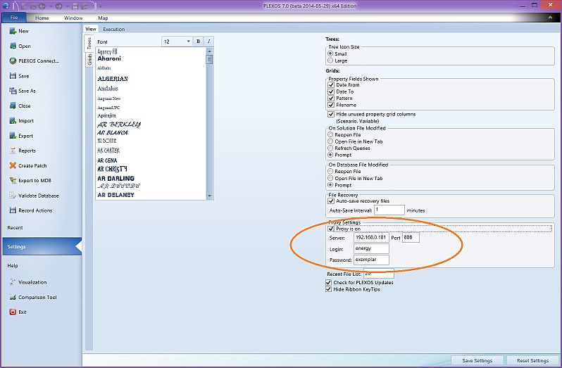
When PLEXOS runs on a PC connected to the internet via proxy, user has to make sure that proper credentials are recorded in Proxy sections of application settings.
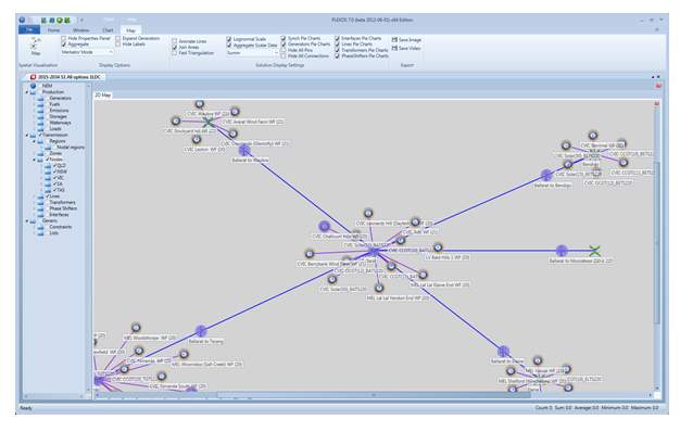
2. Solution Map Layout
Solution map visualization can be accessed by opening the solution of a model, click on the Map tab and select Spatial Visualization. This functionality is only relevant if latitude and longitude coordinates have been assigned to some or all of the objects in a model prior to execution. Objects and memberships cannot be edited in this area of PLEXOS, they can be visualized to a map and the activity of the model can be observed over time with a geographical perspective.
Spatial visualization utilises the Microsoft Bing Map, the application needs an internet connection to access the Bing map and online spatial services. The program confirms access to Bing website and opens the Map visualization window only if the access is available.
2.1. Visualization Window Layout
The visualization window has three areas:
- Tree of filters: Organized as a tree with the same structure as the tree of filters for solution files in the main application.
- Map with visualized objects in the centre.
- Controls for selecting the property to visualize and setting up a query.
2.2. Tree of Filters
As with the input visualization area of the software objects can be put to or removed from the map by checking or unchecking corresponding filters. Enabling a filter puts all related to this filter objects which can be visualized on the map.
Note: Currently only nodes, storages, gas nodes, water nodes, regions, zones, interfaces, phase shifters, lines, gas pipelines, water pipelines, transformers and waterways can be visualized.
Individual objects like nodes, storages, gas nodes, water nodes, lines, gas pipelines, water pipeline transformers and waterways are visualized in the same way as for the input visualization, except when actual data is loaded, these objects will have pie charts on top of their icons.
Currently pie charts display:
- Generation vs available capacity for generators.
- Flow vs Max Flow (or min flow in case flow is negative) for lines, transformers and interfaces.
- Angle vs max (or min) angle for phase shifters.
Generators
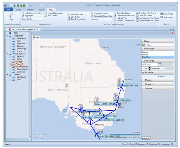
Lines
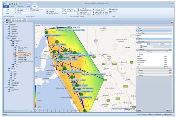
Intraregional Line for SA region (together with price distribution for the region)
Interregional Lines for SA region (together with price distribution for the region)
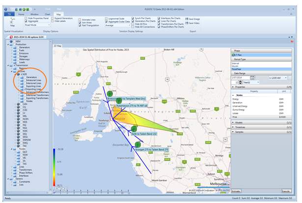
Importing lines for Ade zone (together with price distribution for the zone)
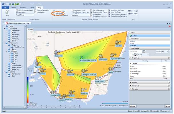
Zones and Regions are displayed as polygon areas coloured according to the selected property distribution described in the Execution section. Areas can be shown as combined (default) or as separate areas (uncheck Join Areas check box on the ribbon Map tab, Solution Display Settings group).
Regions joined (together with price distribution)
Regions displayed separately (together with price distribution)
2.3. Map Controls
Positioning of the map is done using left mouse button and dragging, zoom via the mouse scrolling wheel or keyboard + and - keys
Display Options Group:
Hide Property Panel: Hides/ Displays the property panel on the right hand side.
Aggregate: Toggles the aggregation option (when nodes are close together they are represented by a single aggregate node).
Expand Generators: Arranges all the generators around their node (only possible when a node has 20 generators or less assigned to it).
Hide Labels: Hides/Displays labels of map objects.
Map Mode: User can select from Road Mode (default), Aerial Mode, Faded Road Mode - map tiles become faded to make PLEXOS objects look more distinct, Merkator Mode - grey tiles with no topographic information.
Solution Display Settings Group
Hide All Pins: Hides/ Displays all available Pie Charts.
Hide All Connections: Hides/Displays all selected lines, transformers, waterways, Gas Pipelines and Water Pipelines.
Animate Lines: Turns on the animation effect indicating direction of flow.
Discrete Animation: Displays the changing images over time as a slideshow. Deselecting this option will result in a smoother looking animation with images fading into one another out may take longer to run.
Select Value Levels: Opens a dialogue for selecting and adjusting value levels and colours for data colour fields.
Set Pie Charts: Opens a dialogue for selecting and adjusting value levels and colours for pie charts.
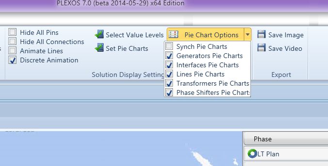
Pie Chart Options: Combo box.
Synch Pie Charts: Updates values for pie charts with solution results (see Execution section).
Generators Pie Charts: Enables displaying Generators Pie Charts.
Interfaces Pie Charts: Enables displaying Interfaces Pie Charts.
Lines Pie Charts: Enables displaying Lines Pie Charts.
Transformers Pie Charts: Enables displaying Transformers Pie Charts.
Phase Shifters Pie Charts: Enables displaying Phase Shifters Pie Charts
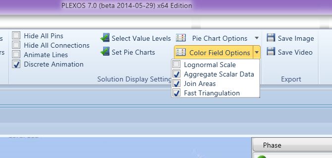
Colour Field Options: Combo box.
Lognormal Scale: Switches to lognormal scale for data visualization.
Aggregate Scalar Data: Switches to aggregation filtering of the data before it is put on the map (close points are represented by aggregated points). This mode works more efficiently on larger models.
Join Areas: Combines displayed areas.
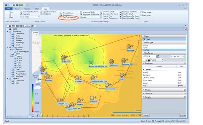
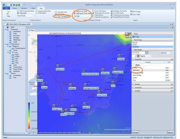
Fast Triangulation: Select the faster triangulation algorithm Delaunay triangulation without creation of regular grid and adding intermediate points.
Aggregation Mode: Combo box. When multiple objects are at one point on the map it is necessary to aggregate the points into one. The following options determine how to handle multiple solutions values.
Display Average: Displays the average value of the aggregated objects.
Display Max: Displays the maximum value of all the objects.
Display Min: Displays the minimum value of all objects.
Display Sum: Displays the summation of all aggregated objects.
Export Group:
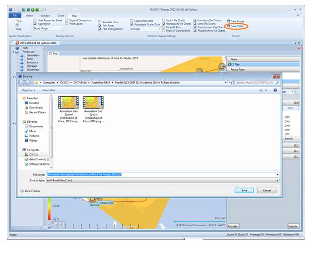
Save Image: Saves an image of the currently displayed map to a .png image file.
Save Video: Saves animation into a .avi file.
Right-click on an object offers the following 4 options:
Select Node: Contains list of nodes aggregated by the pin object.
Select Storage: Contains list of storages aggregated by the pin object.
Select Gas Node: Contains list of gas nodes aggregated by the pin object.
Select Water Node: Contains list of water nodes aggregated by the pin object.
Show Neighbours: Opens a new window on top of the map displaying all the direct connections of the chosen pin object.
Selecting one of these options sets the underlying object as the aggregation centre.
2.4. Execution
Data retrieved for visualization is organised in a similar way to chart visualization, except before selecting the property to visualize an area must be defined (Zone or Region). In order to define the area check one or more Zones or Regions from the filters tree. Then select a property to query and click Execute.
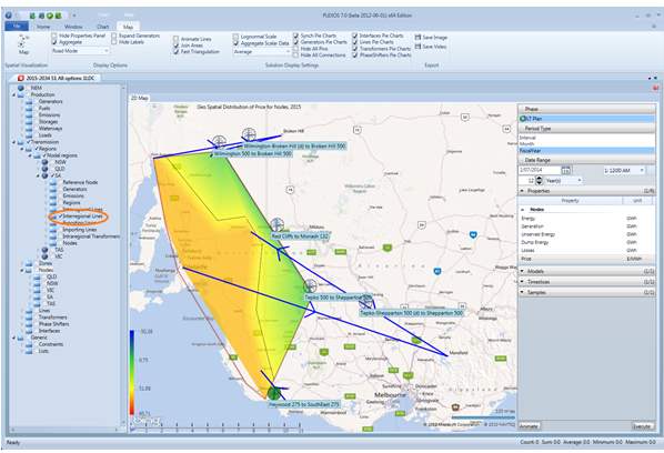
As an example, let's visualize the monthly price for nodes in all available regions for 12 years in LT Schedule phase.
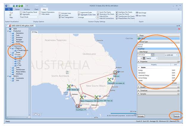
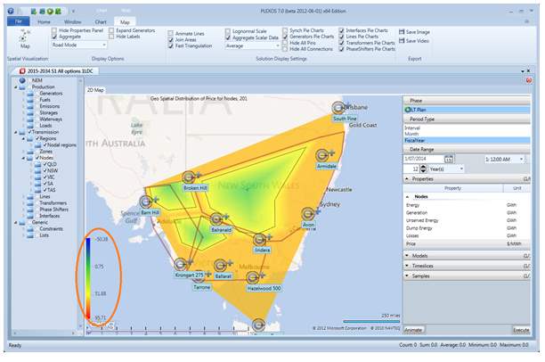
As soon as the Price property is selected, execute the query. The Execute button in the lower right part of the property selection and query filtering controls section. After the price data has loaded, the selected area is coloured according to the price distribution. The colour scale corresponds to the object value and is displayed in the lower left part of the map as a gradient band with several value levels, these value levels are also shown as level lines on the map.
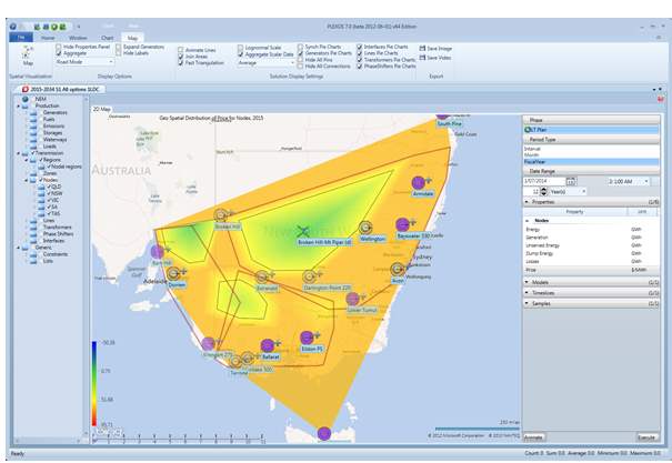
In order to get a picture that included more localised objects and a smoother colour transition (due to usage of fine regular grid), the fast triangulation can be turned off.
For some properties (like Generation) it makes sense to display spatial distribution with different types of values aggregation.
Generation distribution, when nodes with generators are aggregated - their Average generation value is used.
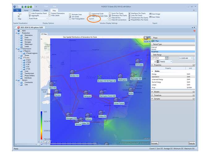
Same Generation distribution but combined generation value is used.
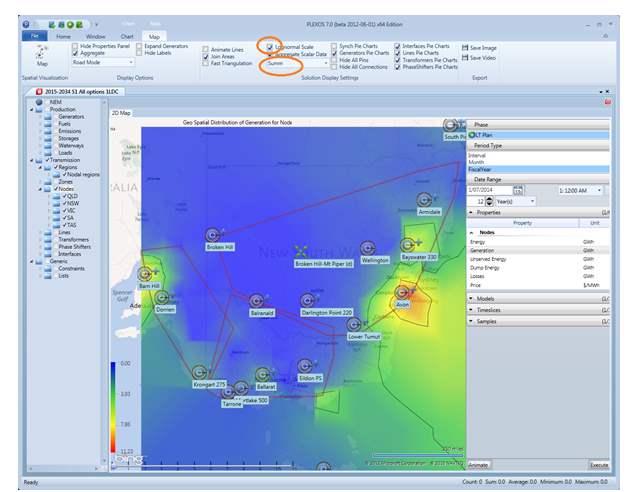
Same Generation distribution, when their combined generation value is used, but in LogNormal scale. After Aggregation or Scale mode is changed user is required to press Execute to apply changes.
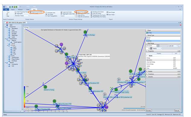
Pie charts for lines and generators, generators are arranged around their nodes (Expand Generators option). When the selected timeline has more than one timestamp, there is a timeline slider near the left bottom of the map, and user can run an animation of the distribution changes over the selected period of time.
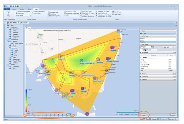
The position of the slider indicates the distribution at that time in the period, the moment of time currently being examined is also reflected in the title of the map. Dragging the thumb along the slider will display the activity of the simulation over different parts of the period.
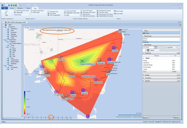
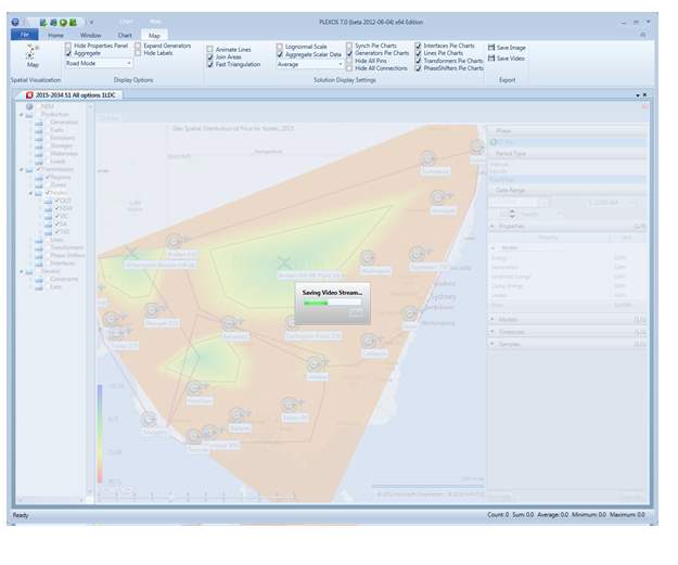
To start the animation feature, press the Animate or Resume button. Animation can be saved as an .avi video file, select Save Video and select location from the open-file dialogue.