Heat Rate Modelling
Contents
- Definitions
- Heat Rate Properties
- Heat Input Function and Convexity
- Separable Programming and Convexity
- Schemes Without Load Point
- Schemes With Load Point
- Heat Rate Formula Conversions
- Heat Rate Output
- References
1. Definitions
The following definitions are used throughout this article:
- The heat input function is given by y = f (x) where y is the heat input (amount of fuel consumed) to produce at megawatt level x for one hour i.e. to produce x megawatt hours of output.
- The marginal heat-rate function is the derivative of the heat input function m (x) = δy / δx
- The average heat rate function is a (x) = f(x) / x
- The term average marginal heat rate refers to the average value of the marginal heat rate function between two points x1 and x2. The average marginal heat rate is equal to the marginal heat rate at the mid-point between x1 and x2 in all cases except if the heat input function is third-order.
- The heat input at a national zero megawatt output is referred to as the no load cost.
Note that the fuel units shown in the examples here are sometimes GJ (giga-joules - Metric) and sometimes MMBTU (million British Thermal Units - Imperial U.S.), but all examples apply to either unit system. Note that "giga" means billion units, and the "M" in "MMBTU" refers to the Roman numeral "M" meaning one thousand, thus "MM" is a way of saying thousand thousands or a million since there is no Roman numeral for million other than the rather awkward convention of writing M with an over-bar.
2. Heat Rate Properties
In the simulator:
- The average heat rate is the property Heat Rate;
- The marginal heat rate is Heat Rate Incr;
- The no load cost is Heat Rate Base.
Where the heat input function is defined as a polynomial function y =
a + bx + cx2 + dx3, the a term (intercept of the heat input function
with the y-axis) is Heat Rate Base, b (linear term) is Heat Rate Incr,
c (quadratic term) is Heat Rate Incr2, and the optional d (tertiary
term) is Heat Rate Incr3.
Broadly speaking the term "heat rate function" might refer to the
marginal or average heat rate function. Both are derived from the heat
input function. There is wide variation on the way heat data are
provided for use in simulation models. For convenience then the
simulator provides six different methods of input by specifying one of
the schemes in Table 1.
Table 1: List of available heat input function schemes.
| Number | Description | Parameters |
|---|---|---|
| 1. | A linear heat input function with constant average and marginal heat rates | Heat Rate or Heat Rate Incr |
| 2. | A linear heat input function with constant marginal heat rate | Heat Rate Base and Heat Rate Incr |
| 3. | A polynomial heat input function | Heat Rate Base, Heat Rate Incr, Heat Rate Incr2, and optionally Heat Rate Incr3 |
| 4. | Pairs of load points and marginal heat rates | Load Point / Heat Rate Incr pairs and optional Heat Rate Base |
| 5. | Pairs of load points and marginal heat rates with no-load cost defined as an average heat rate | Load Point / Heat Rate Incr pairs plus the average Heat Rate |
| 6. | Pairs of load points and average heat rates | Heat Rate / Load Point in multiple bands |
Note that hydro generator efficiency is defined similarly with properties Efficiency Base and Efficiency Incr however the efficiency is the inverse of the marginal heat rate used for thermal generators.
3. Heat Input Function Polynomial
The schemes in Table 1 are simply a method for defining the heat input function. Having received these input the simulator:
- Computes a third-order polynomial fit to the heat input function i.e. no matter which method you use for input the result is always converted to scheme 3 (with exception noted below).
- Divides the space between Min Stable Level and Max Capacity into even length 'tranches' with a tranche reserved for generation below Min Stable Level.
- Calculates a step approximation to the marginal heat rate function based on the average marginal heat rate in each tranche.
The Production settings Fuel Use Function Precision and Max Heat Rate
Tranches control the accuracy and number of tranches used in this
step-wise function. The setting Generator Max Heat Rate Tranches
provides the same control by Generator object. As mentioned above, one
tranche is used for generation below Min Stable Level.
Note that, for input scheme 4, where you define the marginal heat rate
steps at various load points, you can bypass the re-fitting of a
polynomial and force the simulator to use the input marginal heat rate
steps verbatim. This is achieved by setting Generator Max Heat Rate
Tranches to a value less than the specified number of Load Point bands
e.g. if you define three bands of Load Point/Marginal Heat Rate then:
- if Max Heat Rate Tranches ≥ 3 the simulator will fit a polynomial function to the heat input and redistribute the load points evenly between Min Stable Level and Max Capacity; otherwise
- if Max Heat Rate Tranches < 3 the simulator will use all the points and marginal heat rates provided verbatim.
4. Separable Programming and Convexity
The step-wise approximation to the marginal heat rate function is
based on the Fan
Approximation method-see DRAYTON 1997 [1, 2]. This method uses
separable programming to cast the polynomial heat input function as a
linear approximation. Separable programming relies on certain
characteristics both of the marginal heat rate tranches and the
optimization's objective function and other constraints. Firstly the
marginal heat rate 'steps' must be monotonically non-decreasing in
cost. When this is not the case we refer to the function as being
'non-convex'. Secondly their cost should not be zero, nor should any
other constraint or cost in the optimization problem imply that the
marginal value of steps is monotonically non-decreasing. In simple
terms, the optimization must prefer the tranche one marginal heat rate
first, tranche two second, and so on. Any other order and the
approximation will yield an inaccurate modelled heat input function.
To solve this issue the simulator allows you to switch to a variation
of the Fan Approximation that includes additional constraints that
ensure that the tranches are used in order. Because this version
requires integer variables and additional constraints it is not
enabled by default, however warnings from the simulator will indicate
when this integer Fan Approximation might be needed:
- Message 29 is issued whenever the marginal heat rate step function, computed after the fitting of the polynomial, have values that decrease with higher tranche numbers.
- Message 215 is issued whenever the computed Generator Fuel Offtake shows that the heat rate steps have been taken up out of order.
You can switch to the integer Fan Approximation globally by setting
Production Heat Rate Error Method to "Allow Non-convex". The setting
Generator Formulate Non-convex provides the same function for
individual objects.
With this option enabled there is no restriction on the 'convexity' of
the marginal heat rate function, which allows you to model marginal
heat rate functions of practically any shape. Examples occur often
when modelling CCGT plant as
aggregate generator objects.
By default Heat Rate Error Method is set to only warn about the
non-convexity and "adjust" the marginal heat rate function to make it
convex. The adjustment procedure is as follows. Assume the step-wise
marginal heat rate function has steps (tranches) numbered from one
being the tranche starting at notional zero generation to N being the
tranche that runs up to Max Capacity:
- Set n=N-1
- Decrement n. If n=0 then stop.
- If the marginal heat rate in tranche n is less-than-or-equal-to the marginal heat rate in tranche n+1 then go to step 2.
- Set the marginal heat rate in tranche n and n+1 equal to the lesser of the average of values in tranche n and n+1 and the maximum of all values above n+1.
- Go to step 2.
5. Schemes Without Load Point
5.1. Constant Average and Marginal Heat Rates
Figure 1 shows an example of a simple linear heat input function in which the average and marginal heat rate curves are equal i.e. the heat input function has the form y = bx This type of function can be entered by setting the Heat Rate property of the generator as in the following example:
| Property | Value | Metric Units | Value | Imperial Units |
|---|---|---|---|---|
| Units | 1 | - | 1 | - |
| Max Capacity | 250 | MW | 250 | MW |
| Min Stable Level | 70 | MW | 70 | MW |
| Heat Rate | 9.487 | GJ/MWh | 9487 | Btu/kWh |
Note that Heat Rate Incr could also be used here.
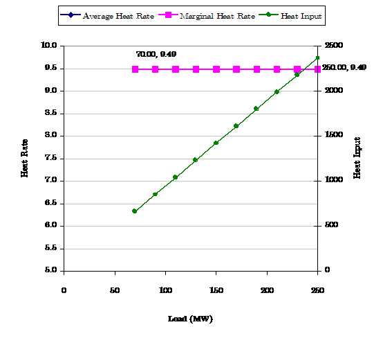 Figure 1: Linear Heat Input Function with Constant Marginal and
Average Heat Rate
Figure 1: Linear Heat Input Function with Constant Marginal and
Average Heat Rate
5.2. Constant Marginal Heat Rate
Figure 2 shows an example of a linear heat input function in the form y = a + bx i.e. with constant marginal heat rate but variable average heat rate. This type of function can be entered by setting the Heat Rate Base and Heat Rate Incr properties of the generator as in the following example:
| Property | Value | Metric Units | Value | Imperial Units |
|---|---|---|---|---|
| Units | 1 | - | 1 | - |
| Max Capacity | 250 | MW | 250 | MW |
| Min Stable Level | 70 | MW | 70 | MW |
| Heat Rate Base | 78 | GJ | 78 | mmBtu |
| Heat Rate Incr | 9.175 | GJ/ MWh | 9175 | Btu/ kWh |
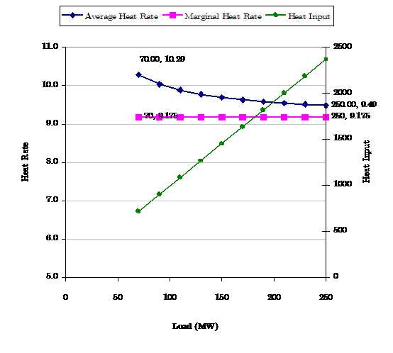 Figure 2: Linear Heat Input Function with Constant Marginal Heat
Rate
Figure 2: Linear Heat Input Function with Constant Marginal Heat
Rate
5.3. Polynomial Heat Input Functions
Figure 3 shows an example of quadratic heat input function. The coefficients are entered using the properties, Heat Rate Base, heat Rate Incr, and Heat Rate Incr2 and in this example:
| Property | Value | Metric Units | Value | Imperial Units |
|---|---|---|---|---|
| Units | 1 | - | 1 | - |
| Max Capacity | 250 | MW | 250 | MW |
| Min Stable Level | 70 | MW | 70 | MW |
| Heat Rate Base | 78 | GJ | 78 | mmBtu |
| Heat Rate Incr | 7.97 | GJ/MWh | 7970 | Btu/kWh |
| Heat Rate Incr2 | 0.00482 | GJ/MWh^2 | 0.00482 | Btu/kWh^2 |
To simulate this curve, PLEXOS will automatically develop a piecewise linear approximation to the quadratic function, and you can specify how many linear tranches are used to make the approximation. This is described below.
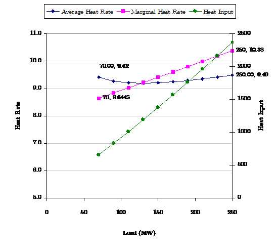 Figure 3: Quadratic Heat Input Function
An extension to this case is to add a third-order coefficient as in the following data and illustrated in Figure 4:
| Property | Value | Metric Units | Value | Imperial Units |
|---|---|---|---|---|
| Units | 1 | - | 1 | - |
| Max Capacity | 250 | MW | 250 | MW |
| Min Stable Level | 70 | MW | 70 | MW |
| Heat Rate Base | 78 | GJ | 78 | mmBtu |
| Heat Rate Incr | 7.97 | GJ/MWh | 7970 | Btu/kWh |
| Heat Rate Incr2 | 0.00482 | GJ/MWh^2 | 0.00482 | Btu/kWh^2 |
| Heat Rate Incr3 | -0..009 | GJ/MWh^3 | -0.000009 | Btu/kWh^3 |
To simulate this curve, PLEXOS will develop a piecewise linear
approximation, but here the marginal heat rate is not monotonically
non-decreasing thus the function is not separable. PLEXOS solves this
problem using MIP as described earlier.
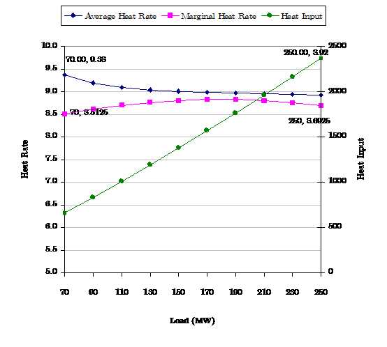 Figure 4: Third-order Polynomial Heat Function
6. Schemes With Load Point
PLEXOS allows for the specification of heat rate functions using
pairs of heat rate (either marginal or average) along with megawatt
load points. The following sections illustrate three methods of input
based on the quadratic heat input function in Figure 3 i.e. these all
produce the same outcome but use different combinations of input
variables. These methods allow the input of heat rate functions that
do not take simple functional forms like those in the preceding cases.
Note that the Load Point may take any value and can overlap or skip
parts of the 'normal' operating range of the unit if required.
Further, as with the polynomial functions, PLEXOS does not require
that the marginal heat rates are monotonically non-decreasing, thus
any set of values can be entered.
The user can also specify separate heat rate functions for different timeslices.
In such a case, it should be ensured that the number of bands remains the
same across all timeslices and the heat rate and load point information
for all bands must be input.
The following properties are common to all the examples:
| Property | Value | Units |
|---|---|---|
| Units | 1 | - |
| Max Capacity | 250 | MW |
| Min Stable Level | 70 | MW |
6.1. Marginal Heat Rates With Intercept
The Heat Rate Base is
specified along with multiple pairs of Load Point and Heat Rate Incr.
Heat Rate Base is the intercept of the heat input function with the
y-axis. Heat Rate Incr is the marginal heat rate at the mid-point of
the band not at the Load Point itself. In this method, the data are
describing the steps of a marginal cost function that PLEXOS should
use to model the generator's heat input function and PLEXOS will use
the function verbatim.
An example for the function show in Figure 3 is:
| Property | Value | Units | Band | ||||||
|---|---|---|---|---|---|---|---|---|---|
| Heat Rate Base | 78 | GJ/hr | 1 | ||||||
| Load Point | 70 | MW | 1 | Heat Rate Incr | 8.3074 | GJ/MWh | 8307.3 | Btu/kWh | 1 |
| Load Point | 90 | MW | 2 | Heat Rate Incr | 8.7412 | GJ/MWh | 8741.2 | Btu/kWh | 2 |
| Load Point | 110 | MW | 3 | Heat Rate Incr | 8.934 | GJ/MWh | 8934.0 | Btu/kWh | 3 |
| Load Point | 130 | MW | 4 | Heat Rate Incr | 9.1268 | GJ/MWh | 9126.8 | Btu/kWh | 4 |
| Load Point | 150 | MW | 5 | Heat Rate Incr | 9.3196 | GJ/MWh | 9319.6 | Btu/kWh | 5 |
| Load Point | 170 | MW | 6 | Heat Rate Incr | 9.5124 | GJ/MWh | 9512.4 | Btu/kWh | 6 |
| Load Point | 190 | MW | 7 | Heat Rate Incr | 9.7052 | GJ/MWh | 9705.2 | Btu/kWh | 7 |
| Load Point | 210 | MW | 8 | Heat Rate Incr | 9.898 | GJ/MWh | 9898.0 | Btu/kWh | 8 |
| Load Point | 230 | MW | 9 | Heat Rate Incr | 10.0908 | GJ/MWh | 10090.8 | Btu/kWh | 9 |
| Load Point | 250 | MW | 10 | Heat Rate Incr | 10.2836 | GJ/MWh | 10283.6 | Btu/kWh | 10 |
6.2. Marginal Heat Rates with Average at Min Stable Level
The Heat Rate is specified at the Min Stable Level along with
multiple pairs of Load Point and Heat Rate Incr. Heat Rate is the
average heat rate at Min Stable Level and is provided only on the band
1 Load Point. The first Load Point must always be at Min Stable Level
and the last must be at Max Capacity. The Heat Rate Incr is the
marginal heat rate at the mid-point of the band.
An example for the function show in Figure 3 is:
| Property | Value | Units | Band | ||||||
|---|---|---|---|---|---|---|---|---|---|
| Load Point | 70 | MW | 1 | Heat Rate | 9.4216 | GJ/MWh | 8307.4 | Btu/kWh | 1 |
| Load Point | 90 | MW | 2 | Heat Rate Incr | 8.7412 | GJ/MWh | 8741.2 | Btu/kWh | 2 |
| Load Point | 110 | MW | 3 | Heat Rate Incr | 8.934 | GJ/MWh | 8934.0 | Btu/kWh | 3 |
| Load Point | 130 | MW | 4 | Heat Rate Incr | 9.1268 | GJ/MWh | 9126.8 | Btu/kWh | 4 |
| Load Point | 150 | MW | 5 | Heat Rate Incr | 9.3196 | GJ/MWh | 9319.6 | Btu/kWh | 5 |
| Load Point | 170 | MW | 6 | Heat Rate Incr | 9.5124 | GJ/MWh | 9512.4 | Btu/kWh | 6 |
| Load Point | 190 | MW | 7 | Heat Rate Incr | 9.7052 | GJ/MWh | 9705.2 | Btu/kWh | 7 |
| Load Point | 210 | MW | 8 | Heat Rate Incr | 9.898 | GJ/MWh | 9898.0 | Btu/kWh | 8 |
| Load Point | 230 | MW | 9 | Heat Rate Incr | 10.0908 | GJ/MWh | 10090.8 | Btu/kWh | 9 |
| Load Point | 250 | MW | 10 | Heat Rate Incr | 10.2836 | GJ/MWh | 10283.6 | Btu/kWh | 10 |
6.3. Average Heat Rates
Multiple Load Point and Heat Rate pairs are specified. Heat Rate is the average heat rate at each Load Point. The Load Point values may take any value and can overlap or skip parts of the 'normal' operating range of the unit if required. Thus, in this method, the data are describing points on the heat input function and PLEXOS will generate a piecewise linear model of the marginal heat rate function from these data.
Note: When using Heat Rate and Load points - the inputs will be approximated with a polynomial first and then tranches are created
An example for the function show in Figure 3 is:
| Property | Value | Units | Band | ||||||
|---|---|---|---|---|---|---|---|---|---|
| Load Point | 70 | MW | 1 | Heat Rate | 9.4216 | GJ/MWh | 9421.6 | Btu/kWh | 1 |
| Load Point | 90 | MW | 2 | Heat Rate | 9.2705 | GJ/MWh | 9270.5 | Btu/kWh | 2 |
| Load Point | 110 | MW | 3 | Heat Rate | 9.2093 | GJ/MWh | 9.2093 | Btu/kWh | 3 |
| Load Point | 130 | MW | 4 | Heat Rate | 9.1966 | GJ/MWh | 9196.6 | Btu/kWh | 4 |
| Load Point | 150 | MW | 5 | Heat Rate | 9.213 | GJ/MWh | 9231.0 | Btu/kWh | 5 |
| Load Point | 170 | MW | 6 | Heat Rate | 9.2482 | GJ/MWh | 9248.2 | Btu/kWh | 6 |
| Load Point | 190 | MW | 7 | Heat Rate | 9.2963 | GJ/MWh | 9296.3 | Btu/kWh | 7 |
| Load Point | 210 | MW | 8 | Heat Rate | 9.3536 | GJ/MWh | 9353,6 | Btu/kWh | 8 |
| Load Point | 230 | MW | 9 | Heat Rate | 9.41775 | GJ/MWh | 9417.75 | Btu/kWh | 9 |
| Load Point | 250 | MW | 10 | Heat Rate | 9.487 | GJ/MWh | 9487.0 | Btu/kWh | 10 |
7. Heat Rate Formula Conversions
To manually convert heat rate functions between formats, start by
computing the heat input (in GJ or MMBTU) at each load point. The
average heat rate function is simply the heat input at the load point
divided by the generation at the point. The incremental function
starts by computing the heat input at min stable level (either as an
average heat rate using the Heat Rate property, or as the No Load
input as Heat Rate Base), and then computing the incremental heat
input for the incremental generation. The incremental heat rate is
then the change in heat input from point n to point n-1 divided by the
change in generation from point n to point n-1.
Always remember unit conversion in the Imperial system. Because heat
rates are expressed in BTU/kWh. Heat input in MMBTU is computed as the
product of generation (MWh) times heat rate (BTU/kWh) times 0.001. The
metric system units do not require conversion.
Our Heat Rate examples above show the units of GJ/MWh = 1000 BTU/kWh.
This is a convenience for the examples only, the actual conversion
factor is 1055.06
8. Heat Rate Output
The following outputs are based on the step-wise approximation to the marginal heat rate function:
- Generator No Load Cost
- Generator Cost Price
- Generator Offer Quantity
The following outputs relate to the heat rate at the given Generator Generation level:
- Generator Marginal Heat Rate
- Generator Average Heat Rate
9. References
- G.R. DRAYTON. Coordinating Energy and Reserves in a Wholesale Electricity Market, Doctoral Thesis, University of Canterbury, New Zealand. 1997.
- G.R. DRAYTON. The Fan Approximation. Drayton Analytics Research Paper Series.