Performance in LT Plan
Contents
- Introduction
- Step Size
- LDC Type and Blocks
- Problem Size
- Linear Versus Integer Optimal
- Transmission Iterations
- Performance Settings
- Advanced Diagnostics
1. Introduction
LT Plan seeks to optimize the capacity expansion and production of the system over long periods of time e.g. 20-30 years. This involves the formulation and solution to large scale mathematical programming problems. LT Plan and the Performance and Transmission settings provide many 'levers' to control the size and number of problems solved. It is important then to understand these options so that you can find the 'right' settings that will solve the LT Plan in good time and with the level of accuracy required.
2. Step Size
In order to find the best combination of new builds, retirements, and production decisions over the entire planning horizon, LT Plan ideally needs to be able to 'see' (optimize) across that horizon in one optimization 'step'. By default LT Plan is configured to solve this way, which guarantees the capacity expansion and production is optimal with respect to events across the planning horizon.
If a single step optimization is too large or slow to solve you can instead solve the planning horizon in several equal-sized steps. This control is on the LT Plan settings dialog:
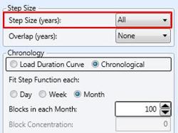
The default setting of All means the complete planning horizon will be solved as a single simulation step. So if the horizon, for example, is defined like this:
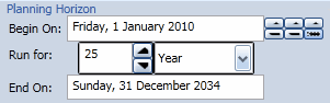
Then in this case a single step spanning 25 years will be simulated. The alternative is to solve in multiple steps. Note though that the steps must be of equal length, so to solve a 25 year span the only practical option would be 5 steps each of 5 years. But if the number of years is flexible these options might be better:
- 3 steps of 8 years each (27 year Horizon)
- 4 steps of 7 years (28 year Horizon)
- 2 steps of 13 years each (26 year Horizon)
In general, the longer the individual steps the better the solution.
3. LDC Type and Blocks
As shown in the LT Plan settings above, the resolution of load duration curves (LDC) can be configured. Again, the more LDC blocks, the better accuracy, but in most cases you will need to control the number of blocks, and frequency of LDC to limit the problem size to a solvable level. The total number of LDC blocks per simulation step is:
- For monthly LDC: Blocks x 12 x years in step
- For weekly LDC: Blocks x 52 x Years in Step
- For dailyLDC: Blocks x 365 x Years in Step
For example, a 25-year horizon solved with monthly LDC each with 12 blocks will have 12 x 12 x 25 = 3600 blocks ('periods') in total.
4. Problem Size
The size of the mathematical programming problem increases approximately linearly with the number of years in each step, and the total number of LDC blocks. LT Plan problems can be very large, but unlike ST Schedule, you generally are solving the problem only once, with perhaps a few iterations (see Transmission Iterations below). When PLEXOS begins to solve LT Plan it will report the size of the optimization 'task' in the log and to the screen like this:
--------------------------------------------------------------------------------------------------------------------------------
Task:  Columns .......656,622  Integers ..........921  Rows ..........460,273  Cones ...............0  Non-zeros  .....1,376,596
 --------------------------------------------------------------------------------------------------------------------------------
The key measure of 'size' is the number of non-zeros. This means the number of coefficients in the matrix being solved. The mathematical programming solvers used by PLEXOS vary in their capabilities for solving large problems, but in general problems up to 3 million non-zeros should be solvable on most solvers and computers including 32-bit computers. Between 3 - 10 million will require a 64-bit computer with perhaps 4 - 8 GB RAM, but problems this size are still in the 'normal' range. Over 10 million is difficult to solve in general and will depend on the case.
5. Linear Versus Integer Optimal
As described in the Capacity Expansion Planning article, integer variables are used to represent the decision to build (or not build), or retire (or not retire) a generation or transmission project: with the exception of Interfaces which are always expanded in a linear fashion. Just as in the above example the number of integers compared to the overall 'size' of the problem is very small. This means that even very large integer models can generally be solved in a tractable amount of time. However, where the solver being used is not integer-capable, or cannot handle the size of problem being solved, it may be necessary to revert to linear optimization of expansion decisions. This is controlled by the following LT Plan setting:
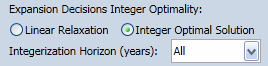
There are several ways to control the extent to which integer variables are applied in LT Plan:
- The above switch that turns on/off use of integers by default for expansion decisions.
- The "Integerization Horizon" which controls how many years of the horizon have integer variables versus linear. For example you might want to integerize only the first 10 years decisions, and accept linear thereafter.
- The properties Generator Expansion Optimality, and Line Expansion Optimality which allow you to set integer or linear by project.
Having decided to what extent decisions will be integer versus linear, it is imperative to set Performance settings suitable for the LT Plan. See the section Performance Settings below.
6. Transmission Iterations
If your system contains a transmission network you firstly have choices over the level of transmission detail solved. LT Plan includes a setting that determines the transmission model used:
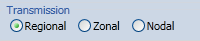
The default Regional setting means that any transmission network inside each Region object will be aggregated by discarding the intra-regional Nodes and connecting all Generators and other resources and loads to a single notional regional reference node. No constraints will be considered inside each Region, nor will intraregional losses. The Zonal option works the same but uses Zone objects as the basis for aggregation. The Nodal option preserves the network without any aggregation.
Note that you have finer control over Regional aggregation with the Region Aggregate Transmission property. Note also that in Nodal mode LT Plan will perform a full Optimal Power Flow. In fact the full range of transmission constraints is available including security constraints and contingencies.
In all cases, the default behaviour of LT Plan is to resolve transmission constraints in an iterative manner, first solving unconstrained, and then adding constraints as they are required.
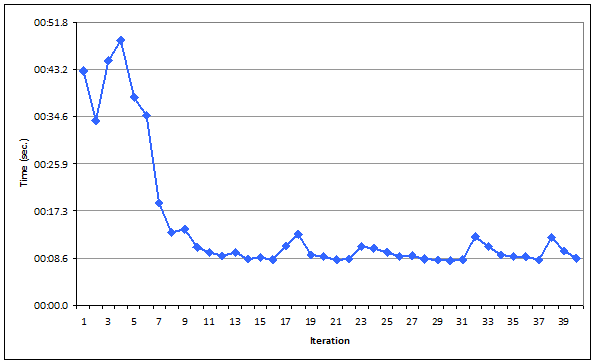
The log file and screen show the iterations like this:
 Transmission Iteration     1. Enforced  3008 Limits. Time: 0:00:42.889
 Transmission Iteration     2. Enforced  2072 Limits. Time: 0:00:33.850
 ...
 Transmission Iteration    55. Enforced    83 Limits. Time: 0:00:10.070
 Transmission Iteration    56. Enforced    17 Limits. Time: 0:00:08.607
The iterations stop when n more transmission limits are added. The following chart shows a typical set of iterations and the time taken to solve each.
In systems with many 100 or 1000's transmission Nodes (or Regions/Zones in that mode) or those solving with Contingencies, there may be no option but to solve iteratively: due to the large number of potential constraints. However, in smaller/more aggregated systems, and especially when Contingencies are ignored the number of limits can be small enough that it is more efficient to solve the initial LT Plan model with all potential limit enforced 'upfront'.
The Transmission settings include a switch for modelling limits 'upfront' as shown here:
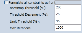
Turning on this option will prevent iterations in the LT Plan (except for Contingencies) and, especially for integer optimization, this can greatly improve performance.
Note that finer control of the 'upfront' setting is available using the Line Formulate Upfront, Transformer Formulate Upfront, and Interface Formulate Upfront properties.
7. Performance Settings
Selecting appropriate Performance settings can have a big effect on runtime for LT Plan. For integer optimization, the default settings are rarely the best. The following is a more suitable selection of options:
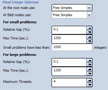
The following have been changed from default values:
- MIP Root Optimizer: The default of Interior Point is changed to Free Simplex. You should test the two options to find the best for your model.
- MIP Relative Gap: The gap allowed before declaring the current best integer solution 'optimal' is raised from the default of 0.01% to 0.1%.
- MIP Max Time: A time limit is set so that the integer solver does not spend too much time simply trying to prove optimality. Note this setting should be tuned to suit your model. If you are solving very large problems then you may need to allow several hours solve time.
- MIP Maximum Threads: Multiple threads can greatly improve performance of large integer models.
For linear optimization you may want to test the effect of changing from Interior Point to Free Simplex.
8. Advanced Diagnostics
To find out more information about what elements of your model are consuming space in the mathematical programming problem you can enable the Diagnostic Task Components setting. This additional report will also tell you the total number of potential transmission constraints, which can be useful for deciding if the 'upfront' transmission option is viable.