Transmission - Shift Factors

Contents

1. Introduction
2. Phase Angle
3. Single Slack Bus
4. Distributed Load Slack
5. Distributed Generation Slack
6. Example
7. Single Slack Bus
8. Distributed Load Slack Case

1. Introduction

In total there are three available methods for allocation of slack for shift-factor calculations:

1. Single Slack Bus (default)
2. Distributed Load Slack
3. Distributed Generation

Within the latter option there are two alternatives, discussed below. The slack bus selection is labelled "Shift Factor (PTDF) Method" in Figure 6.

2. Phase Angles

From the linearized DC-OPF we have that:

θ = [X]P

where:

• θ is the vector of node phase angles
• P is the vector of node injections
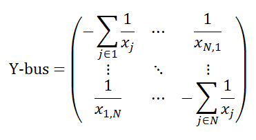
• [X] is the inverse of Y-bus: the N x N matrix of network impedances

The off-diagonal coefficients of Y-bus are simply the susceptance for the line between the buses. The on-diagonal terms are the sum of all path susceptances into the bus:

Given [X] (the inverse of Y-bus) we can calculate the node phase angles for any set of injections P . From the phase angles we can then compute the flow on any path in the network. This is the way shift factors are computed.

However, directly inverting Y-bus is not practical, for all but the smallest systems because the computational effort required scales exponential with N. Thus, PLEXOS instead:

1. Creates the set of equations A_x=b, where A is the Y-bus matrix, x is a vector of bus phase angles (in radians) and b is a vector of bus injections (in megawatts)
2. Solves A_x=b for each row i in x, with the vector b having zero values except for unity in row i
3. Computes the shift-factor for each path j, PTDF_(i,j)=a_(i,j)x(x_j-x_j)

Note that each "projection" (solution of Ax=b) yields a set of shift-factors for all paths with respect to injections at each bus i. Thus we must compute one projection for each injection point (Node that has either generation or load). In a large system this could mean solving thousands of these projections; however, the relatively simple set of linear equations is solved quickly and efficiently by modern Simplex codes. PLEXOS reports progress during the calculation of shift factors with log messages like:

On the other hand, if the node phase angle bound is enabled, the phase angle for each bus will be calculated by

θ = [X]P

Where [X] matrix is now recognized as the angle reference matrix, calculated by assigning a single angle reference node in the network.

3. Single Slack Bus

The single slack bus is identified by setting the Node [Is Slack Bus] attribute to true. If no Node is identified PLEXOS chooses the first Node in the network. The shift-factors are computed by eliminating from Y-bus the row and column corresponding to the slack bus, then solving the system of equations Ax=b for each injection point.

4. Distributed Load Slack

For an incremental injection at a bus, the slack is distributed across all load buses in the system in proportion to their loading in a given reference case. The reference nodal load is equal to Node Load Participation Factor multiplied by the Region Load. Note that Region Reference Load is a static property and thus only one pattern of loads can be used to set the load slacks. If Region Reference Load is not defined, the Region Load defined in the first period of the planning horizon is used instead.

The solution method here is similar to the single slack bus case, but instead of forming Ax=b with A as Y-bus, no rows or columns are eliminated i.e. A is N×N in size. The matrix A is singular, thus we set one of the phase angles (x) to zero. The choice for this node is made by first solving the system 'freely' and then setting the node with lowest angles to zero. The system is then resolved successively for each row of x that is an injection (generation or load) node. At each projection i the b vector contains unity less the slack allocation in row i and the set of (negative signed) normalized loads across the rows corresponding to the load nodes. Thus the sum of elements in b is always zero.

5. Distributed Generation Slack

For an incremental injection at bus i the slack is distributed across all the generation nodes. The proportion of slack assigned to each node is decided according to the Transmission [Slack Bus Method] which for generation slack has two options:

1. Distribute in proportion to the generator capacity
2. Distribute in proportion to input reference generation levels (using the Generator Reference Generation input)

The solution method here is similar to the distributed load slack case.

6. Example

Consider the 7-Node network. The system has three regions with loads as in Table 12. The nodes have the load participation factors in Table 11. Note that in the absence of any Node settings its [Is Slack Bus] attribute to "Yes" Node "1" will default to the slack bus. The transmission line impedance and thermal limits data are shown in Table 11. Note, in linearized DC-OPF, Line Reactance only is considered in computing shift factors, though Resistance is used to compute losses during the simulation. The Generator capacity data are shown in Table 14.

7. Single Slack Bus

For the purposes of computing shift-factors all that is required to form the Y-bus matrix are the line impedances shown in Table 13. The system of equations representing Y-bus is as follows:

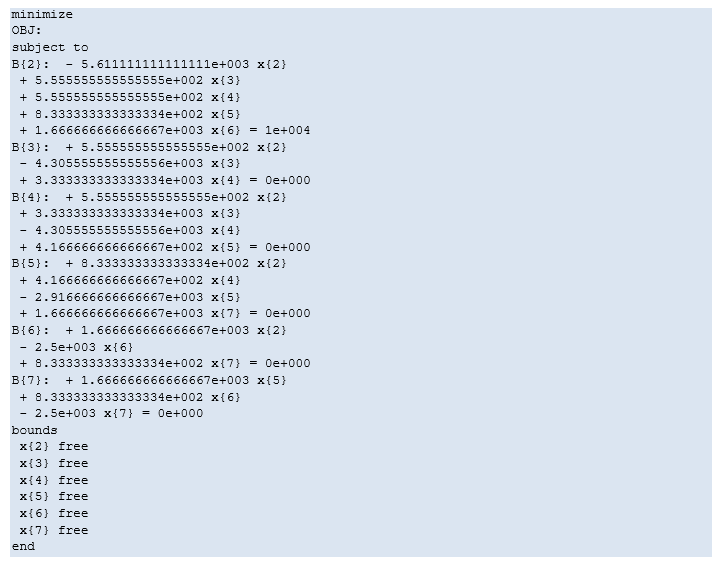
Note the use of the injection (10000 MW) at Node "2". This is the LP used to compute the shift factors for all paths for injections into that node. The large injection is used (rather than unity) to improve numerical stability: an injection of unity would produce very small phase angles and introduce rounding errors into the shift factors.

The process of solving this set of equations with injections at each point in sequence yields the set of shift-factors in Table 17. The PLEXOS log file shows the following line once the shift factor computation is complete:

There are seven "projections" done, one for each injection point (load or generation point). Interpreting the first few rows of Table 17, an incremental injection at bus "2" and simultaneous withdrawal at bus "1" (the slack bus) will decrease the flow on the path "1_2" by 0.865, the path "1_3" by 0.135, the increase the flow on path "2_3" by 0.06027698, and so on.

8. Distributed Load Slack Case

Here PLEXOS forms the 7x7 matrix of network impedance but does not eliminate any equations: thus the initial system of equations solved is:

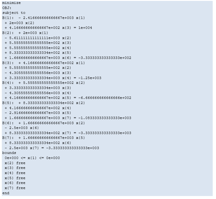
The right-hand side values equal the (negative of the) normalized slack, equal to the proportion of total system load that occurs at the bus in the reference load case. Solving this set of equations for injections at each generation bus yields the set of shift-factors in Table 18.