Cournot Class
| Description: | Nash-Cournot game |
See also Cournot Property Reference for a detailed list of properties for this class of object.
Introduction
Cournot objects are used to provide input to and solution information from the Nash Cournot game, which is enabled via the Competition Equilibrium Model setting.
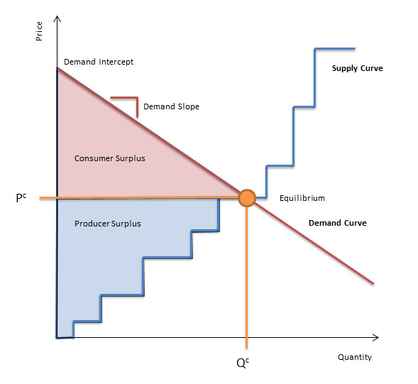
The input properties of a Cournot object define a linear demand function as illustrated in Figure 1:
pi = Pi0 + Ki0qiwhere:
pi is the priceqi is the demand
Pi0 and Ki0 are respectively, the Demand Intercept and Demand Slope in Region i.
The Region collection identifies which Region the demand function applies.
Elasticity versus Demand Curve
Defining the demand function using a Cournot object is an alternative and more detailed approach than simply using either the Competition Default Elasticity or the Region Elasticity. However this demand curve is not easy to compute a priori since it relies on knowing the price and quantity point around which the elasticity applies. To obtain the demand curve parameters from a simulation, using elasticity as an input, such that the same demand curve can be entered as input to a subsequent simulation e.g. when computing the Customer Benefits of a transmission augmentation or market rule change, follow this approach:
- Create Cournot objects, one for each Region and create the memberships to those Regions.
- Do not define Demand Intercept or Demand Slope or use a Scenario to drop them from the running Model.
- Set either the 'global' Competition Default Elasticity or the Region Elasticity appropriately.
- In the Report object for the running Model select output of Demand Intercept or Demand Slope for MT Schedule.
- Run the simulation with the Nash-Cournot game enabled and MT Schedule.
You will now have the parameters of the demand functions used for each Cournot object available in the solution database (or text files if you chose this output option). Now use these data as input for the next simulation by defining Demand Intercept and Demand Slope. Simulations that include these data will now use the Cournot-defined demand function rather than the equilibrium input, since the Cournot demand curve overrides elasticity.
Solution
The Cournot class also reports many useful properties such as the Consumer Surplus and Producer Surplus. Refer to Figure 1 for an explanation of these values in the context of a linear demand function and stepwise supply function. A complete list of outputs is shown in the Cournot Property Reference.

Figure 1: Supply and Demand Curves and Equilibrium