Model Class

Description:

Collection of data scenarios that define a model to be evaluated

See also Model Property Reference for a detailed list of properties for this class of object.

When PLEXOS executes a simulation it executes one or more Model objects.

Model Components

Each Model contains all the information required to define a simulation including:

• Horizon
• Report

Optionally, a Model can link to one or more data Scenarios so that data can be switched in/out of the Model.

Finally a Model can have its execution interleaved with that of another Model. See below for details.

Simulation Phases

There are four main simulation algorithms which are referred to as 'simulation phases'. A Model can have relationships to one of each of:

1. LT Plan
2. PASA
3. MT Schedule
4. ST Schedule

To enable a phase simply add one of these objects into the corresponding Model collection e.g. ST Schedule will run if the Model's ST Schedule collection has one member. The simulation phases will be executed in the above order with certain solution data automatically passed between them. For example LT Plan passes down the optimal expansion plan, and PASA passes the maintenance plan down.

Simulation Settings

Simulation settings are divided into functional groups and implemented as objects. Properties on these objects control the various algorithms and formulation detail of the simulation phases. These are controlled by associating the Model with objects of the Settings class as in the following table:

Class	Description
Stochastic	Settings related to stochastic Variables and Monte Carlo simulation
Transmission	Settings for the transmission and Optimal Power Flow model
Production	Settings related to the Production Cost model e.g. Generator modelling
Competition	Settings related to the modelling of competition and Mark-up
Performance	Settings related to the select Solver
Diagnostic	Settings controlling simulation diagnostics

If no settings object is associated with the Model, default values of those settings will apply - see the settings class pages for details. The settings objects associated with the running Model override those defaults, and further, you may override the settings applied to any given simulation phase by associating a settings object with the simulation phase object. For example, you might want different levels of diagnostic to apply to MT Schedule compared to ST Schedule. This is achieved by associating different Diagnostic objects with the phase object(s), in this case to either or both of MT Schedule Diagnostic or ST Schedule Diagnostic. Other examples include changing the Unit Commitment Optimality setting by phase e.g. linear in some phases and integer in others, or even changing the selected solver or solver tolerances by phase.

Batch and Parallel Execution and Executing in Connect

You may execute more than one Model in a 'batch' simply by selecting multiple Models from the graphical user interface Execute form as shown in Figure 1.

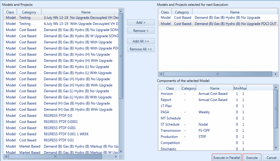Figure 1: Execute Form

Pressing Execute begins execution of the selected Models in a batch, with each Model run in sequence. Execute in Parallel divides the selected Models into multiple parallel batches. The number of parallel runs is set in PLEXOS Settings.

If you have PLEXOS Connect installed you also have the option to Execute to Connect, which allows you to send the execution to one of multiple client computers on your network.

By default execution of Models takes place in a separate console window as in Figure 2. You can choose a different style of execution window via PLEXOS Settings.

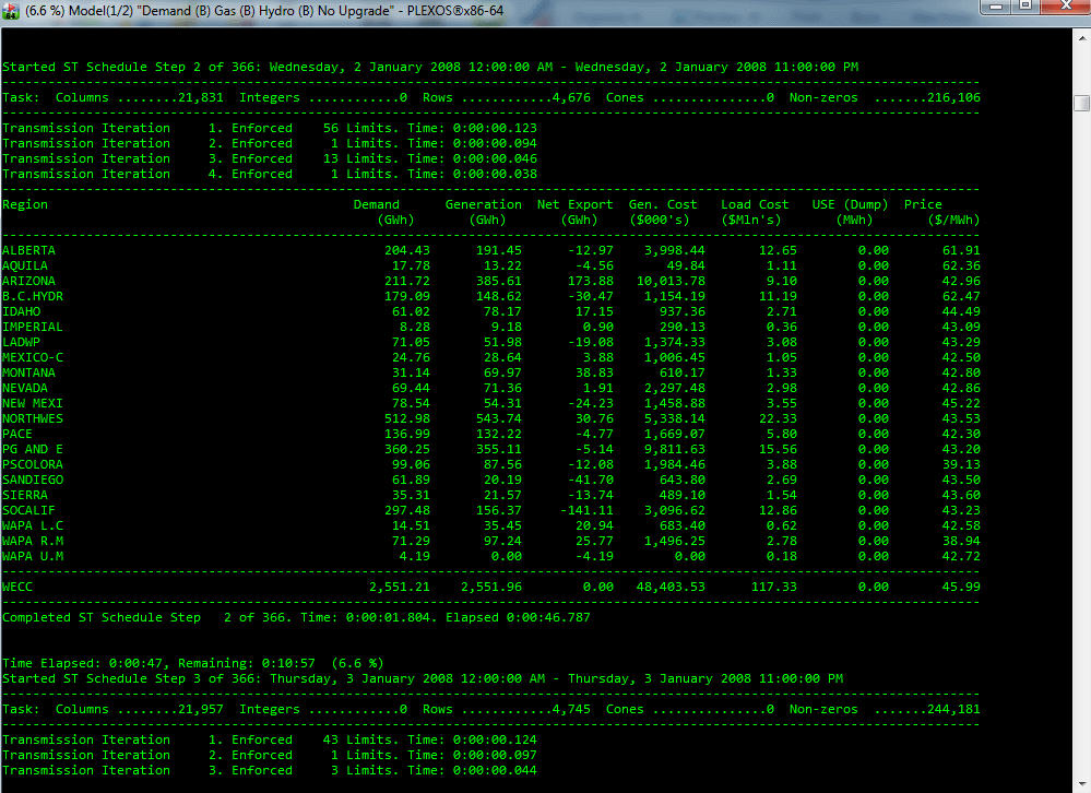Figure 2: Console Execution Window

Passing Data between Models

Often it is required that one Model read the solution of another Model as part of its input. For example, simulating a balancing (real-time) market where certain decisions are made by another "day-ahead" Model. This can be achieved by running the two Models in a batch, with the "day-ahead" Model running first, the "real-time" second. The order of execution defaults to Model category then name alphabetically, but this can be overridden with the Execution Order setting. The data are passed by writing of solution flat files (text files) by the "day-ahead" Model and reading of those files with Data File objects. See the Report class for details and the article Balancing Markets for examples.

Interleaved Run Mode

Interleaved run mode is a more sophisticated way to link the solutions of one Model with another. In interleaved mode the simulation steps of ST Schedule of two Models are run 'in step' and solution data are passed both ways. For example the "day-ahead" Model can pass unit commitment and any other required information to the "real-time" Model to cover the first day of the simulation. Once the 'real-time' Model has completed the first day it will pass initial conditions for Generator and Storage objects back to the "day-ahead" Model. This process is illustrated in Figure 3. In that example the "day-ahead" Model runs in steps of one day at a time, whereas the "real-time" runs in steps of an hour at a time. The resolution (Periods per Day) of the Models need not be the same e.g. "day-ahead" might run with hourly resolution, whereas "real-time" might be at a 15-minute resolution. Any combination is acceptable and data passed between the Models is upscaled/downscaled automatically. For more information on upscaling and downscaling of data see the topics in Data File.

Invoke the interleaved mode by adding the "real-time" Model (the second Model) into the Interleaved collection of the "day-ahead" Model. The data passed from the "day-ahead" Model is decided by setting up references to the text solution data of that model in the "real-time" Model in exactly the same way as you would to run those Models in a batch. However, you do not need to actually write out those flat files since data will instead be passed in memory i.e. the Report Write Flat Files setting can be 'off' when in interleaved mode.

Users can suppress commencing forced outages in the "day-ahead" model by setting the SuppressInterleaveOutages undocumented parameter to true. This will not affect the forced outages from being modeled in the "real-time" model, or commenced forced outages from being modeled in the "day-ahead" model.

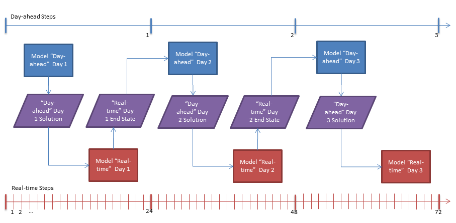Figure 3: Flow Diagram of Interleaved Run Mode

Note: Both "day-ahead" (first) and "real-time" (second) models must use the same stochastic methods and sample counts. Also Stochastic Method set to "Parallel Monte Carlo" under ST Schedule is not supported for interleaved runs.

Performance Tips

The simulator uses the selected Solver to solve the mathematical programming problems generated during the simulation. Considerable scope is available via Model Performance settings and the Horizon to control the speed of the simulation.

The simulator divides the Horizon into steps. Each step is solved with one mathematical programming problem. The steps are always of equal length (this improves efficiency). Horizon and/or LT Plan, MT Schedule settings control the size of each step and hence the number of steps solved. In general, shorter steps are faster, but there is also overhead in having too many steps. These aspects are discussed in the following section.

Solution Speed

LT Plan is usually configured to solve the entire Horizon as a single step but there are three controls that determine the size of the simulation step:

1. LDC Type which can be either day / week / month;
2. At a Time which defaults to the entire horizon but can be configured to any number of years; and
3. Overlap which allows one step to overlap the next.

Using the Chronology setting LT Plan can be switched between using load duration curves to reduce the complexity of the simulation or preserving the original chronology. A chronological simulation includes more detail especially in unit commitment and technical constraints for generators.

When using load duration curves (LDC) the number of blocks in each curve can be reduced over the duration of the horizon to improve performance and allow the detail of the simulation to focus on the near-term. These detail parameters are controlled by Block Count and Last Block Count.

The PASA algorithm has two resolution settings: daily or weekly steps. The daily option is preferred for accuracy but if the algorithm is running slow on a very large system you may set the resolution to weekly.

In MT Schedule there are four parts to the resolution:

1. Step Type which can be either day / week / month;
2. At a Time which defaults to one year at a time;
3. LDC Type which can be either day / week / month; and
4. number of Block Count (time periods) used in each step.

You can improve performance by increasing the step type, decreasing the number of blocks, or reducing the step size.

MT Schedule can also switch Chronology modes.

For ST Schedule the steps are controlled by settings on the Main.Horizon where you choose:

1. Step Type which can be either minute / hour / day / week; and
2. step size.

You can improve performance by reducing the length of the simulation step e.g. solve a week in seven steps each of one day, rather than one step of a week.

The speed of ST Schedule is also affected by the interval length. You can improve execution speed tremendously by increasing the length of each interval. In addition you can choose between running a full chronology or solving only a typical week per month.

ST Schedule can also make use of a 'look-ahead' period which improves unit commitment decisions while allowing a shorter step size. The look-ahead resolution can be lower than the resolution of the main step e.g. you might solve the horizon in daily steps with hourly resolution with an additional day look-ahead at a three-hourly resolution.

Using the above options you can 'tune' the simulation such that the mathematical program size lies in the 'sweet spot' for the selected solver. See the article Optimizing Performance for a detailed discussion of the available solvers and options.

Memory Use

In general it is good practice to try to keep the total memory charge of the computer under the physical limit of memory while running the simulation. If the simulator uses more memory than this, the computer will waste a lot of time swapping data in and out of virtual memory.

The simulator uses memory in three ways:

1. To store working data such as a temporary copy of input data that is needed in each simulation step - these data are already heavily compressed to minimize memory use, but you can control how text data are handled.
2. To store data that will be used to create the summary solution data e.g. daily summary results - the selections here affect memory and #Output Size">output size.
3. The solver uses memory to store and solve mathematical programming problems.

Output Size

The performance of the simulator is sensitive to the amount of output data that needs to be written to the solution database. Also the format of output is important with zipped-XML being the fastest and most compact format.

Before running any model, it is advisable to review all output data settings, and disable any output that is not required. Use the following process as a guide:

1. Decide whether or not any summary data are required at all from the simulation. Summary data are those at the daily, weekly, monthly, or annual level and are calculated automatically for you during the simulation (if requested). Normally it is convenient to get the simulator to produce summary data to at least one of these levels e.g. annual data, but in some cases data is really only needed at the trading period level. Switching off all summary data greatly improves simulation performance in all phases of the model.
2. Daily data is especially onerous to store and calculate across a long horizon, so try to limit the number of categories of output data you need.
3. Annual data are the most efficient to report and will result in very little overhead across a long horizon.
4. If trading period level data are required, try to reduce the number of properties written to the bare minimum especially for classes with a large number of objects. Trading period data takes up the most space in the solution database.
5. Finally, consult the table below for some suggested set up for various databases.

Dry Run Mode

A "dry run" is one where all functions of a normal run occur except for solution of the mathematical programming problems in each simulation step. A dry run can be used to check that all input data are working as expected and that Variable sampling is functioning. All output data are written and thus this mode can also be used to refine size/performance of the output. Dry Run mode is invoke via the a hidden parameter.

Feasibility Repair

Infeasible problems can be relaxed automatically, allowing recovery from these situations and the simulation to continue. All the supported solvers provide this functionality and simulator exploits it so that it may continue regardless of infeasibilities. If an infeasibility is encountered during the course of a simulation the following steps are taken:

1. The mathematical problem is written to disk and diagnostics of the infeasibility are printed to the screen and log file (for use in diagnosing the infeasibility offline).
2. The solver is called to determine which constraints require relaxation in order to solve the infeasibility.
3. The problem is modified to reflect the recommendations made by the solver, and the modifications are reported to the screen and log file, and the repaired problem is written to disk.
4. The simulation step is rerun using the modified problem and the simulation continues normally. A warning is issued about the infeasible problem. The following is an example report:

 
             MOSEK PRIMAL INFEASIBILITY REPORT.    Problem status: The problem is primal infeasible
             The following constraints are involved in the primal infeasibility.
             Index     Name             Lower bound     Upper bound     Dual lower     Dual upper  
             167     NodNetInjDef_1{168}     3.000000e+001     3.000000e+001     0.000000e+000     1.000000e+000  
             335     NodPwrBal_1{168}     0.000000e+000     0.000000e+000     0.000000e+000     1.000000e+000  
             839     Con_tx{168}         5.000000e+001     5.000000e+001     0.000000e+000     1.000000e+000  
             1007     PhyMinTotGen_import{168} 9.900000e+001     NONE         1.000000e+000     0.000000e+000    
             The following bound constraints are involved in the infeasibility.    
             Index     Name             Lower bound     Upper bound     Dual lower     Dual upper   
             167     NodUSE_1{168}         0.000000e+000     NONE         1.000000e+000     0.000000e+000  
             839     ConUnd_tx{168}         0.000000e+000     NONE         1.000000e+000     0.000000e+000    

             MOSEK FEASIBILITY REPAIR REPORT.    
             Sum of Violations 31.9200000000001    

             The following constraints were repaired.    
             Index     Name         Lower bound     Repaired     Upper bound     Repaired   
             839     Con_tx{168}     5.000000e+001     5.000000e+001     5.000000e+001     6.900000e+001    
                

In the above example the repair information says that the user-defined Constraint "tx" should have its right-hand side increased from 50 to 69.

Note that:

• The simulator sets priorities for the constraints and bounds in the simulation. User defined Constraints are relaxed first, then other bounds such as transmission limits, then other lower bounds. The weights used to decide which constraints are relaxed and in what order can be written to a diagnostic file and can also be set by the user via an input XML file.
• Feasibility repair can be a slow process on large models and can consume large amounts of memory; therefore you should review the infeasibility repair information and make appropriate adjustments to the simulation problem in order to avoid needed these repairs during the simulation.
• In some rare cases the repaired problem might not be sensible due to the choice of constraints that are relaxed thus feasibility repair information should always be reviewed carefully to assess the impact of the repair on the quality of the results. If the infeasibility does not appear to be related to user-defined data or generic Constraints, report the issue to the Support Team as it may relate to errors in the underlying simulation formulation.