Constraint Class

Description:

Generic constraint

The RHS Custom type is used to define multi-annual or other special timeframes such as quarterly constraints.

The left-hand side coefficients (a_(i,j)) are defined according to the simulation variable they multiply against. So for example if a term is to appear against Generator Generation you first add the Generator involved to the Generators collection of the Constraint then set the Generators Generation Coefficient property equal to the a_(i,j) value. You can include any number of objects in the Constraint collections and set coefficients in virtually any combination required.

The Constraint Property Reference describes the Constraint properties and all available left-hand side coefficients.

1.2. Creating Constraints

Constraints are defined with three basic elements:

• The sense of the constraint
• The right-hand side constant
• The left-hand side coefficients

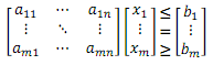
Constraints are always expressed in one of the following forms:

A x ≤ b
A x ≥ b
A x = b

The term, A, represents the matrix of all left-hand side coefficients, x represents the vector of decision variables that appear in the constraints, and b is the vector of right-hand side constants. In matrix form this can be illustrated as:

The constraints cannot have decision variable coefficients (terms) on the right-hand side. These must be entered as left-hand side coefficients by simply swapping signs: an example is given below.

Suppose a constraint is in the form:

Line Flow ≤ 100 - 0.01 Generator Generation

The terms in the constraint must be rearranged to group all decision variable coefficients on the left-hand side:

Line Flow + 0.01 Generator Generation ≤ 100

Note further than the term on the Line Flow here is implicitly unity, and thus the following constraint is mathematically equivalent:

-Line Flow - 0.01 Generator Generation ≥ -100

Notice how multiplying all coefficients through by minus one also causes the sense of the constraint to flip. You are free to define constraints in the way that is most convenient.

Each Constraint object should have its Sense property defined. The constant right-hand side (b vector) values are set by the properties in Table 1 depending on the period of the constraint:

• whereas RHS, RHS Hour, RHS Day, .... , RHS Year define a sequence of constraints; one for each

period type in the horizon;

• RHS Custom defines a single constraint that notionally spans the entire horizon; more

on this later.

A Constraint object has several collections whose members determine what terms appear on the left-hand side of the constraint. The left-hand-side terms refer to decision variables in the formulation.

Because more than one term is allowed to appear in the constraint for each type of object, these coefficients default to a value of zero, and so you must set the coefficients even if they are unity. For example, to include the Generation of a Generator on the left-hand side of a constraint:

1. Add the Generator to the Constraint Generators collection
2. Set the Generation Coefficient property on that membership to 1.

Before you create a Constraint you must first enable the Constraint class in Configuration and any left-hand side coefficient properties you intend to set. For the below example the configuration required looks like that in Figure 1 which shows the necessary property selections in red highlight.

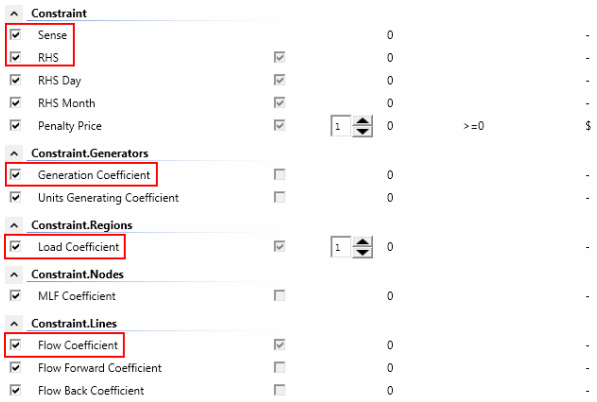Figure 1: Example Configuration for Constraint Class

1.3. Example

In the Australian NEM, the regional transmission model is supplemented with 'generic' constraints. These constraints approximate the effect of transmission thermal, voltage and stability limits not explicitly accounted for in the market's regional transportation model. An example of this situation is the thermal transmission limit for exports from the "NSW" region to the "Snowy" region, which is stated as:

"NSW to SNOWY" Flow ≤ 1561 - 0.014 "NSW1" Demand + 0.107 x "MP1-2" Generation + 0.0107 x "WW7-8" Generation

To enter this constraint through the user interface:

1. Create a Constraint object, e.g. named "Max Flow NSW to SNOWY (Thermal Limit)".
2. In the Constraint dialog, double-click the Regions collection and using the Membership Editor, add the Region "NSW1". Return to the Constraint form.
3. Likewise add the Generator objects "MP1", "MP2" and "WW7", "WW8" to the Constraint Generators collection, and the Line "NSW to SNOWY" to the Constraint Lines collection.
4. Select "≤" as the Sense. Note that the Sense property is displayed as one of "≤", "≥", "=" but these are stored in the database as - 1, 1, 0 respectively.
5. The right hand side constant is 1561 and is set with the RHS property.

The coefficients on flow, load and generation are set on the Constraint Lines, Constraint Regions and Constraint Generators collections respectively. The coefficients must be entered as if they appeared on the left-hand side of the constraint; therefore:

• Line "SNOWY" has Flow Coefficient 1
• Region "NSW1" has Load Coefficient 0.014
• Generator objects "MP1-2" and "WW7-8" have Generation Coefficient of -0.107.

The finished constraint should look like that in Figure 2.

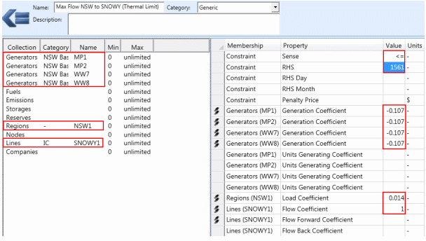Figure 2: Example Transmission Constraint

With the RHS property defined this Constraint object will generate one constraint (row) in the formulation for each interval of the simulation (half-hour in the Australian NEM case)

If you print the LP file for this case, the following rows appear in the file:

 Con_Max Flow NSW to SNOWY (Thermal Limit){1}: LinFlow_NSW to SNOWY{1} - 0.107 GenLoad_MP1{1}
                          - 0.107 GenLoad_MP2{1} - 0.107 GenLoad_WW7{1} - 0.107 GenLoad_WW8{1}
                          <= 1468.082 
                 Con_Max Flow NSW to SNOWY (Thermal Limit){2}: LinFlow_NSW to SNOWY{2} - 0.107 GenLoad_MP1{2}
                          - 0.107 GenLoad_MP2{2} - 0.107 GenLoad_WW7{2} - 0.107 GenLoad_WW8{2}
                          <= 1466.304 
                 Con_Max Flow NSW to SNOWY (Thermal Limit){3}: LinFlow_NSW to SNOWY{3} - 0.107 GenLoad_MP1{3}
                          - 0.107 GenLoad_MP2{3} - 0.107 GenLoad_WW7{3} - 0.107 GenLoad_WW8{3}
                          <= 1464.82 
                

...

 Con_Max Flow NSW to SNOWY (Thermal Limit){24}: LinFlow_NSW to SNOWY{24} - 0.107 GenLoad_MP1{24}
                          - 0.107 GenLoad_MP2{24} - 0.107 GenLoad_WW7{24}
                          - 0.107 GenLoad_WW8{24} = 1467.382
                

Note how the left-hand side does not contain any term related to Region Load but instead the right-hand side constant changes dynamically. This is because the Load Coefficient term can be pre-computed and shifted to the right-hand side. This kind of substitution of coefficients for their equivalent constant term on the right-hand side is performed automatically.

All of the properties here can be made dynamic and thus change across time e.g. the RHS might change according to time of year.

Note that transmission constraints such as this are by default not added to the formulation 'up front' but instead are held in reserve and checked and added dynamically during the simulation. This is usually the most efficient way to enforce these constraints because it avoids 'bloating' the formulation with many likely redundant constraints. You can optionally force all transmission constraints to be added up front with the Transmission Formulate Upfront toggle.

1.4. Units of the Right-hand-side

For interval constraints (those defining Constraint RHS), the units of right-hand-side are unscaled. For example if you are constraining:

• The maximum flow on a transmission line, the units are megawatts
• The generation of a generator, the units are megawatts
• The number of units generating at a generator, the units are number of unit

For constraints that span multiple periods (those defining Constraint RHS Day, RHS Week, etc) as well as RHS Hour the units for the right-hand-side match those in the reported summary output. So for constraints on:

• Fuel the unit is TJ (or GBTU)
• Generation the unit is GWh
• Emissions the unit is tonne (or ton)
• Units generating or units started the unit is number of units with no scaling
• Capacity built, installed or available the unit is megawatts

1.5. Multi-annual, seasonal and other Special Constraints

The property Constraint RHS Custom allows for the specification of constraints that span any period of time such as multiple years (multi-annual constraint) or a subset of time such as a season or quarter.

Figure 3 shows an example of a multi-annual constraint on the emissions produced by a Generator. Note the use of Date From and Date To on the constraint coefficient and how this defines the timespan over which the constraint applies.

A constraint like this that spans multiple years requires a simulation step size large enough to span the constraint. This can be achieved by either using LT Plan which defaults to a single step across the planning horizon, or by customising the MT Schedule step size so that it spans a long enough period.

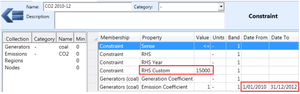Figure 3: Example multi-annual constraint

Another interesting application of dates or timeslices on the constraint coefficients is for defining seasonal constraints. Figure 4 is an example of a constraint on generation across the summer season. Using RHS Year creates one constraint each year, but the Timeslice applied to the coefficients means that only the required season is included.

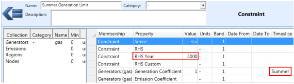Figure 4: Example seasonal constraint

2. Filtering Using Memberships

A number of the left-hand side coefficients, like Generators Emission Coefficient will encompass every Emission produced by the Generator objects included in the Constraint. Often you will need to apply the constraint across a subset of those objects e.g. just one of the Emission objects rather than all. This can be achieved by including the membership of the Emission in the Constraint Emissions collection but without setting any coefficients. This is interpreted as a "filter membership".

An example is shown in Figure 5 where the emissions of a set of generators are under constraint using Constraint Generators [Emission Coefficient], but because the generators produce multiple emissions it is necessary to filter the coefficients by including the Constraint Emissions "CO2" membership with no coefficient set.

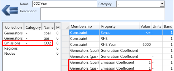Figure 5: Constraint using Filtering Membership

The membership types listed in Table 2 can be used to filter the objects included in a Constraint.

Table 2: Memberships that can be used to filter constraint coefficients

Collection	Example
Reserve.Constraints	Generators Filter the Generator objects for Constraint Reserves [Provision Coefficient]
Fuel.Constraints	Fuels Filter the Fuel objects for Constraint Generators [Fuel Offtake Coefficient]
Emission.Constraints	Emissions Filter the Emission objects for Constraint Generators [Emission Coefficient]
Constraint.Companies	Companies Filter the Company objects for Constraint Emissions [Production Coefficient]

3. Switching Constraints On and Off

Every Constraint object defined is assumed to exist for the entire simulation period. Even if the right-hand-side value is defined only after a user-defined Date From, the constraint, with default zero right-hand-side constant, will still appear in every period before that date. But userdefined constraints often need to be made conditional in one of a number of ways. You can:

• include a constraint only if a given Scenario is included in your Model; or
• make a constraint active only in certain time periods; or
• include a constraint only in a given phase or phases of the simulation; or
• apply a Constraint only when certain conditions are active in the simulation; or
• apply an offset to a constraint so that it is 'swamped' (made always slack) when a

condition occurs.

Commonly these latter two methods would apply to generic constraints such as transmission nomograms, or transmission network security constraints. These constraints often require different forms under different conditions - examples are shown below.

3.1. Switched by Scenario

It is a general rule that a Constraint will be dropped from the formulation if no right-hand side properties (or 'constant terms') are defined/included in the executing Model. Right-hand-side is thus the 'key' property for a Constraint in that it is used to switch the constraint on/off by including/excluding the property definition. Constraint objects can be associated with Scenario objects in the same manner as any other input.

To specify that a constraint appears only in Model runs that include a given Scenario, simply 'tag' all right-hand-side property values with that Scenario name (in the Scenario column). An example is given in Table 3. Here the Constraint changes from being a daily constraint to monthly according to the defined Scenario tags. To apply the constraint in a Model, include one of the Scenario objects "Hydro Daily" or "Hydro Monthly".

Table 3: Constraint switched by Scenario

Constraint	Property	Value	Units	Band	Data File	Scenario
ARDNA	RHS Day	0	-	1	DAILY.csv	Hydro Daily
ARDNA	RHS Month	0	-	1	MONTHLY.csv	Hydro Monthly
ERNE	RHS Day	0	-	1	DAILY.csv	Hydro Daily
ERNE	RHS Month	0	-	1	MONTHLY.csv	Hydro Monthly
LEE	RHS Day	0	-	1	DAILY.csv	Hydro Daily
LEE	RHS Month	0	-	1	MONTHLY.csv	Hydro Monthly
LIFFEY	RHS Day	0	-	1	DAILY.csv	Hydro Daily
LIFFEY	RHS Month	0	-	1	MONTHLY.csv	Hydro Monthly

Note that a warning is not issued if a Constraint appears in the Model with no right-hand side values defined because the switching of constraints in/out of models using right-hand side with Scenario is normal procedure. Note that excluded constraints will not appear in the solution database. In the above example, no default right-hand-side is defined so if neither Scenario is included in a Model, the Constraint will not be formulated.

3.2. Switched by Time Period

In some situations, a constraint may be active only after a certain date and/or inactivate after a certain date. Tagging the right-hand side with a Scenario name can only switch the constraint in and out of the entire horizon, not selected parts.

There are three ways to switch constraints in/out by time period:

1. swamp the right-hand side value so the constraint can never bind in periods it is not required; or
2. allow zero-penalty violations of the constraint in periods it is not required; or
3. tag all left-hand side coefficients with Date From, Date To and or Timeslice so that only the needed time periods are collected.

Table 3 shows an example of an upper-limit constraint being swamped by a large right-hand side value prior to the period in which the constraint applies. Tables 4 and 5 show examples of allowing zero-priced violations of the constraint prior to the period in which the constraint applies using the Constraint Penalty Price property, which creates a soft constraint (see below).

Table 3: Swamping a Constraint

Property	Value	Units	Date From
Sense	≤	-
RHS	9999	-
RHS	500	-	1/01/2004

Table 4: Relaxing with Zero Penalty Price and Soft Constraint Otherwise

Property	Value	Units	Date From
Sense	≤	-
RHS	500	-
Penalty Price	0	-
Penalty Price	5000	-	1/01/2004

Table 5: Relaxing with Zero Penalty Price and Hard Constraint Otherwise

Property	Value	Units	Date From
Sense	≤	-
RHS	500	-
Penalty Price	0	-
Penalty Price	-1	-	1/01/2004

You have two choices when relaxing the constraint with Penalty Price:

• use a high positive value during the 'active' period; or
• set a price of -1 which indicates that the constraint is 'hard' during that period.

The approach of allowing using a large positive price when the constraint is active has the disadvantage that large penalty values may cause numerical instability in the solver and slow execution time. In general consider a penalty price of 1E+6 for interval constraints or 1E+9 as upper limits on what is safe to use without causing numerical instability.

However, it is not always straight-forward to swamp a constraint, especially equality constraints, thus where possible use the swamping method, otherwise use the penalty method with -1 for hard constraint or keep the Penalty Price as low as you need to make the constraint bind without violations.

3.3. Switching by Simulation Phase

Constraints can be switched in and out of each phase of the simulation using the properties Constraint Include in LT Plan, Include in PASA, Include in MT Schedule, and Include in ST Schedule.

Note further that constraints using coefficients dedicated to capacity expansion planning will only be formulated in LT Plan.

3.4. Conditional Constraints

The simulator includes a special class of objects called Variable, which can be used with Constraint to produce truly conditional constraints, i.e. constraints that activate automatically when some user-defined set of conditions occurs. These conditions can be static or they can be dynamic, but they cannot be optimized.

NOTE: To have a Constraint switch on/off according to an optimized decision you must use the Decision Variable class.

Once the required Variable objects have been defined they can be applied to Constraint objects to create conditional constraints. To make a Constraint conditional, simply add the appropriate Variable object(s) to the Constraint Conditions collection.

By default, when multiple conditions are included in a constraint, the conditions must all be active simultaneously to activate the Constraint. Thus the Variable objects are combined with AND logic. You can change this behaviour and make OR conditions by setting the Constraint Condition Logic property.

The output property Constraint Hours Active gives feedback on when constraints have been activated and how often.

3.4.1. RHS Changes by Condition

Condition objects can also be used to modify the right-hand side (constant term) of a constraint when they are active. The property is added to the right-hand-side when the constraint is active.

Table 6: Adjusting RHS using a Condition

Constraint	Property	Value	Units
V-SA MAX	Sense	≤	-
V-SA MAX	RHS	400	-

Constraint	Lines	Property	Value	Units
V-SA MAX	V-SA	Flow Coefficient	1	MW
V-SA MAX	TORRB > 2 UNIT	RHS Coefficient	100	-

Here the limit for flow on the transmission line "V-SA" is 400 in all periods except if the Variable "TORRB > 2 UNITS" is active, in which case the limit is 400 + 100 = 500 MW.

3.4.2. Conditional Constraint Properties

Conditions may also be used to change the right-hand-side or coefficients in a constraint according to which condition is active at any one time as in the following example:

Table 7: Conditional Property

Constraint	Property	Value	Units	Band	Date From	Date To	Timeslice	Condition
V-SA MAX	RHS	550	-	1				Load < 2500
V-SA MAX	RHS	480	-	1				Load < 3000, Load >= 2500
V-SA MAX	RHS	400	-	1				-

It is important not to 'overlap' conditional data. In the above example two conditions are AND together on the value of 480 so that this statement does not overlap with the previous condition. If we simply applied the condition "Load < 3000" to the value, both conditional values would be active if the load were less than 2500, creating some ambiguity as to which value to use.

NOTE: Overlapping conditions are difficult for the simulation engine to detect and no warning is issued.

4. Soft Constraints

By default, constraints are 'hard' constraints, i.e. they can potentially cause infeasibilities in the simulation. Although the simulator can automatically recover from infeasibilities the execution will be slow during feasibility repair and consume a lot more memory so it is always desirable to create constraints that are always feasible.

For maximum simulation speed and if you are certain that a user-defined constraint will never generate an infeasibility then it is best to leave it to be modelled has a 'hard' constraint. There are situations, however, in which constraint violations could, and should, be allowed as in the section Switching Constraints On and Off. The Penalty Quantity and Penalty Price properties of the Constraint object allow you to set up violation in multiple bands. In the simplest case use the Penalty Price alone. Constraint violations will be priced at this incremental value and the amount of violation is notionally unlimited. This is illustrated in the following example:

Table 8: Uniform Penalty Function

Property	Value	Units	Memo
Sense	≤	-
RHS	2000	-	TJ
Penalty Price	5000	-	$/TJ

Note the use of the Memo field to label the units of the Constraint terms.

If you wish to setup a number of penalty bands each with a different penalty price, use Penalty Price in combination with Penalty Quantity as in the following example. Note that the units for Penalty Quantity are always the same as those of the right-hand-side.

Table 9: Step Penalty Function

Property	Value	Units	Band	Memo
Sense	≤	-	-	-
RHS	2000	-	1	TJ
Penalty Quantity	500	-	1	TJ
Penalty Quantity	1000	-	2	TJ
Penalty Price	5000	-	1	$/TJ
Penalty Price	15000	-	2	$/TJ

5. Implied Constraints

The simulator provides a number of 'shortcut' properties that allow you to create a Constraint with a simple property definition rather than having to create a Constraint object and add the coefficients, etc. These special properties are converted to Constraint objects by the simulation engine at runtime.

Examples of implied constraints include Generator Max Energy Day and Emission Max Production Year. Refer to the property pages for each class for more examples.

Note that these implied Constraint objects appear in the formulation but are not reported on in the solution database. They are limited in that they can only formulate constraints on the single object the property is defined on, thus if you wish to define constraints that include terms for several different types of object you will need to create your own Constraint objects. For example a constraint on an Emission will encompass all Generators and/or Fuels that produce that Emission, so if you need to limit the constraint to a subset of those sources you will need to use a Constraint.

Note: Hourly Implied Constraints (e.g. Generator Max Energy Hour) only apply to sub-hourly models i.e. those where Horizon Periods per Day is greater than 24.

6. Constraint Reporting

Table 10 lists the reporting properties for the Constraint class.

Activity is the total of all left-hand-side terms, so for example if the constraint were:

1 x Generator "A" Generation + 1 x Generator "B" Generation ≤ 500

The activity here is the sum of Generator "A" and "B" generation.

The RHS is the constant term, in this case 500. The Slack is the difference between the Activity and the RHS, thus if Activity is 400, the Slack is 100. Note that by convention greater-than-or-equal-to constraints have negative slack.

Violation applies if the constraint defines a penalty function (see Soft Constraints) or if the Constraint has been repaired (see Feasibility Repair). Penalty Cost is the objective function contribution of the violation.

Hours Binding indicates if the Constraint is binding in the period, which is defined as having zero slack and a non-zero Price. Price is the shadow price of the constraint, equal to the optimal value of the dual variable associated with the constraint.

Rental is the shadow price multiplied by the activity and represents the contribution of the constraint to the dual objective function.

Constraint Hours Active indicates if the constraint is included in the formulation. This applies to conditional constraints and to constraints identified as transmission-specific that are added to the formulation dynamically.

Table 10: Constraint Report Properties

Property	Unit	Description
Activity	-	Constraint activity at optimal solution
Slack	-	Constraint slack at optimal solution
Violation	-	Constraint violation at optimal solution
Hours Binding	hrs	Number of hours the constraint is binding
RHS	-	Constraint RHS constant
Price	$	Constraint dual variable value at optimal solution
Hours Active	hrs	Number of hours the constraint is active (according to applied Conditions)
Penalty Cost	$ ($000)	Contribution of penalty violations to the primal objective function
Rental	$ ($000)	Contribution of activity to the dual objective function

7. Feasibility Repair

If any of the mathematical programming problems formulated during simulation is infeasible, an automatic feasibility repair is invoked. The goal of the feasibility repair is to find a repair to the problem that is optimal with respect to the original objective function combined with penalties for violating constraints and/or variable bounds. These penalties are set internally and create a priority list for violations. User-defined constraints are usually the first constraints violated, having the lowest weight.

Whenever possible infeasibilities should be avoided. There is significant overhead in repairing the problem and the repair might not always be 'sensible'. Log messages can help you identify the infeasibility and guide you to the correct solution, which might involve changing Constraint data such as the right-hand-side or adding a Penalty Price to allow violations.

Example

To demonstrate feasibility repair, let's assume the following Constraint is defined:

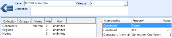Figure 6: Example Infeasible Constraint

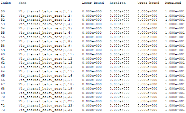
The constraint is clearly infeasible as it is attempting to hold Generator "thermal" Generation below zero. When this is run in a simulation the report below appears:

• The first highlight is the message that appears when a problem is identified by the

solver as infeasible. The style of this message might vary depending upon the solver used, but they key point is that the problem status is "Primal Infeasible".

• In the next section (the Infeasibility Report) a list is given of all constraints and variable

bounds in the problem that might be related to the infeasibility. This is simply a list of those constraints and bounds that have non-zero dual values at the infeasible solution. The true cause of the infeasibility will be listed here, but there may be many other related elements listed.

• After a period of time a Feasibility Repair Report is printed. This presents the solution to

the 'optimal' problem repair if one exists. It lists all constraints and/or variable bounds that have been modified. In this example the violation variables on each of the 24 (hourly) constraints has been modified from zero upper bound to an upper bound of 10. This relieves the constraint and makes the problem feasible.

Constraint objects are always denoted in these reports with the format "Con_<name>{p}" where <name> is the name of the Constraint and p is the period number in the simulation step. The violation variable "Vio_" and slack variable "Slk_" are always included even if the constraint does not define a penalty function.

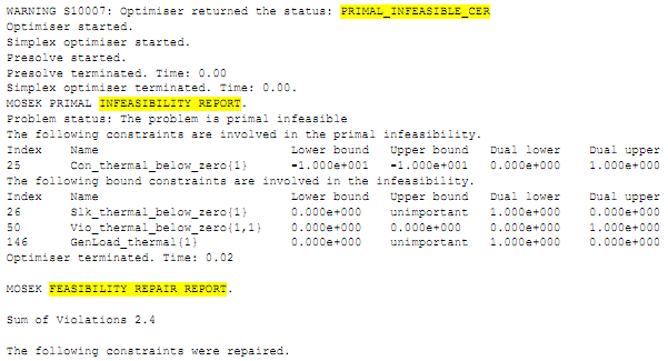
In general not every infeasible problem can be repaired, but if the infeasibility is due only to user-defined constraints then a repair is always possible by relaxing one or more of those constraints. The only reason that such a repair would fail is if the memory required to find the optimal repair is too great.

8. Constraint Decomposition

8.1. Introduction

Inter-temporal constraints such as fuel contract constraints, emission limits, and hydro energy limits are an important feature of electricity market modelling. The simulator solves medium term constraints like this in two phases. In the first phase (MT Schedule), all inter-temporal constraints are formulated directly. To be able to model long horizons like a year in a single model, the MT Schedule uses temporal compression via load-duration curves. In the second phase (ST Schedule) every interval of the horizon (e.g. hour, half-hour, or 5-minute) is modelled in detail but the horizon is divided into a sequence of steps, each having a user-defined number of intervals e.g. 24 hours, a week etc.

8.2. Constraint Period Type

As described earlier, constraints may be defined to apply across days, week, months, years, or multiple years. This behaviour is determined by the particular right-hand side property set: [RHS], [RHS Day], [RHS Week], [RHS Month], [RHS Year], or [RHS Custom]. Only the right-hand side property carries the period type of the constraint and other constraint properties such as [Penalty Quantity] will automatically take the same period type as the right-hand side.

8.3. Inter-temporal Optimization

The simulation is a truly inter-temporal optimization; constraints that sum or relate values across time periods are formulated directly in the optimization, ensuring that all decisions are co-optimized with respect to those constraints, and the constraints are always met optimally or correctly identified as infeasible. This contrasts with many other simulators, which simulate period-by-period and simply record the activity on inter-temporal constraints and take some rule-of-thumb approach to enforcing them. The multi-phase inter-temporal approach is superior because both the physical (primal) and pricing (dual) impact of the constraints are recognised.

However, to solve the simulation problem as an inter-temporal optimization, every constraint must have a time period less-than or equal-to the length of the simulation step size, or put another way the simulation step size must be long enough to 'cover' the longest user-defined inter-temporal constraint. The ST Schedule phase is used to produce the time-sequential (chronological) simulation results. Because even modest sized systems can produce large optimization problems in ST Schedule the simulator is generally configured (via Horizon properties) to solve the horizon in steps of one week or day or in some cases even smaller steps. With each step every interval, e.g. hour, half-hour, 5-minute interval, is modelled.

For example, a one-year simulation is commonly solved as 365 one-day optimizations in ST Schedule. This means that the simulator will create 365 optimization problems each spanning a day and solve these sequentially. Each step will include a full representation of the simulation problem for each interval. In this multi-step scheme, inter-temporal constraints such as annual limits cannot be directly represented - because the maximum span on any one optimization problem is just one day (in this example). One approach to this is to increase the size of the ST Schedule step, e.g. to change the ST Schedule to solve one step of 365 days, i.e. solve the entire simulation problem as a single optimization problem. But, as noted above, this would lead to a single optimization problem that is too large to solve. Thus to keep the size of the ST Schedule to a reasonable level the simulator includes long and mid-term phases (LT Plan and MT Schedule) which work with ST Schedule to decompose long term constraints into equivalent short-term constraints, small enough for ST Schedule to model directly.

8.4. Decomposition Method

The role of the MT Schedule (and to a lesser extent LT Plan) in constraint modelling is to decompose inter-temporal constraints that would otherwise be too long for ST Schedule. The Constraint [Decomposition Method] controls the style of decomposition. You can choose between decomposition of the constraint quantities or decomposition on price. In general quantity decomposition is most appropriate and this is described here.

Example:

Constraint	Property	Value	Units
Annual CO2	Sense	≤	-
Annual CO2	RHS Year	200000000	-

Constraint	Emission	Property	Value	Units
Annual CO2	CO2	Production Coefficient	1	-

This example defines a constraint on annual "CO2" emissions. If the simulation uses ST Schedule in conjunction with MT Schedule, the simulator will use the MT Schedule emissions output to allocate the emission constraint intelligently across the steps of the ST Schedule, e.g. if the ST Schedule step-size is one day then the simulator allocates the (annual) emission constraint limit to ST Schedule days based on the MT Schedule emissions.

Constraint	Property	Year Ending	Value	Units
Annual CO2	Activity	30-JUN-05	171169113.04	-
Annual CO2	Slack	30-JUN-05	28830886.96	-
Annual CO2	Violation	30-JUN-05	-	-
Annual CO2	Price	30-JUN-05	-	-
Annual CO2	Hours Binding	30-JUN-05	-	-
Annual CO2	Hours Active	30-JUN-05	-	-

The table shows the annual summary results for the "CO2" Emission. The total [Activity] is less than the input right-hand side because the constraint is slack, i.e. there are less emissions being produced than limited by the [RHS Year]. The [Slack] output shows the total slack on the constraint for the year.

The [Activity], [Slack], and [Violation] are decomposed to all other reporting periods (interval, day, week, etc). Figure 7 shows the daily activity on the constraint with slack. ST Schedule is set up to run in daily steps so it is this profile of daily constraint activity and slack that is used to create constraints for ST Schedule. The simulator creates these constraints and passes them to ST Schedule automatically as part of a step called the "MT to ST Schedule Bridge".

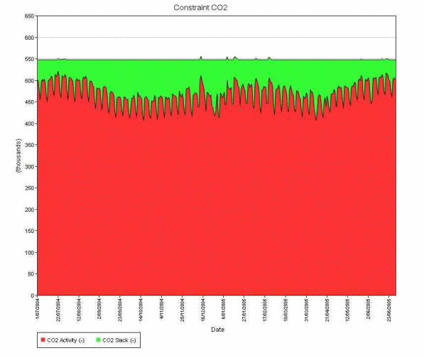
Figure 7: MT Schedule Constraint Activity, Slack, and Violation decomposed to days for slack constrain

Constraints that are slack, or soft constraints that have violation, in MT Schedule have their activity, slack and violation decomposed to the ST Schedule. This ensures that ST Schedule does not mistakenly create binding constraints in each of its steps when the original constraint is slack, or in the case of soft constraints it ensures that ST Schedule allows appropriate violations. The allocation of slack and violation across sub-periods is a non-trivial problem. The simulator optimizes the allocation to produce the smooth distribution shown in Figure 7.

In the case where the constraint has some violation (the properties [Penalty Price] and or [Penalty Quantity] are defined), the allocation of violation follows the constraint activity as shown in Figure 8. Finally, if the constraint is exactly binding (no slack or violation) only the constraint activity and any allowable violation is passed to ST Schedule as shown in Figure 9.

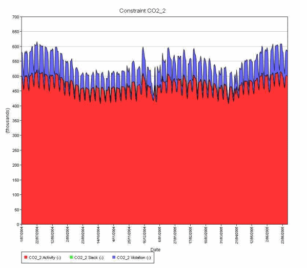
Figure 8: MT Schedule Constraint Activity, Slack, and Violation decomposed to days for constraint with violation

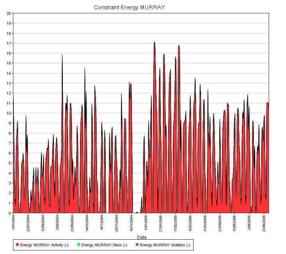
Figure 9: MT Schedule Constraint Activity, Slack, and Violation decomposed to days for binding constraint

Having performed the decomposition of these inter-temporal constraints, the simulator creates the set of constraints to be used in each ST Schedule step. In the emission example, each ST Schedule step will solve using a daily emission limit. The aggregate results for these constraints will equate closely with the annual results from MT Schedule or multi-annual results from LT Plan ensuring that the original limit is obeyed.

Regarding decomposition in general, note the following:

• If a simulation only uses the MT Schedule or LT Plan then the step-size (one year by default) must be set to at least as long as the longest constraint time period, i.e. the MT Schedule step-size should always be sufficiently large to handle all constraints.

• If ST Schedule is used alone then any constraint that has a time period longer than the ST Schedule step size will be dropped from the model prior to execution, and the simulator will issue an appropriate warning. You should enable MT Schedule and/or LT Plan in this case.

• If ST Schedule is configured to use a look-ahead period ahead of each step and there are constraints decomposed from MT Schedule or LT Plan, it is preferred, but not required, that the amount of look-ahead hours are equal to (or a multiple times of) the length of the step type, eg. for a daily step ST, it's better to set the total look-ahead hours as 24, 48 or 72, etc, so the decomposed daily limit will apply to all look-head periods.

9. Constraints on Maximum Value Across Time

9.1. Introduction

Constraint LHS Type controls the way the simulator forms up constraint left-hand side terms. Three types of equations are supported: 'SUM', 'MAXSUM' and 'MAX'. This provides more options for user to model constraints.

9.2. SUM Type

The default type is 'SUM' that LHS value of the equation is the sum of all terms in the left-hand side across the time period.

Example:

Constraint	Property	Value	Units
TotalGen	Sense	≤	-
TotalGen	RHS	400	MW

Constraint	Generator	Property	Value	Units
TotalGen	Gen1	Generation Coefficient	1	-
TotalGen	Gen2	Generation Coefficient	1	-
TotalGen	Gen3	Generation Coefficient	1	-

This example defines a constraint on total generation of three generators. The math equation for each interval can be expressed as below.

TotalGen: Gen1_Load + Gen2_Load + Gen3_Load ≤ 400

Example:

Constraint	Property	Value	Units
TotalGen	Sense	≤	-
TotalGen	RHS Day	900	GW

Constraint	Generator	Property	Value	Units
TotalGen	Gen1	Generation Coefficient	1	-
TotalGen	Gen2	Generation Coefficient	1	-
TotalGen	Gen3	Generation Coefficient	1	-

Once [RHS Day] is defined, the equation will count all the simulation intervals of a day.

TotalGen: ∑_(i)(Gen1_Load_(i) + Gen2_Load_(i) + Gen3_Load_(i)) ≤ 900,000

9.3. MAXSUM Type

The 'MAXSUM' type is for the maximum value of the sum of left-hand side coefficient across the period.

Example:

Constraint	Property	Value	Units
MaxSumGen	Sense	≤	-
MaxSumGen	RHS	800	MW

Constraint	Generator	Property	Value	Units
MaxSumGen	Gen1	Generation Coefficient	1	-
MaxSumGen	Gen2	Generation Coefficient	1	-
MaxSumGen	Gen3	Generation Coefficient	1	-

When using 'MAXSUM' type for interval constraints, it has the same formula as 'SUM' type. This example defines a constraint on sum generation of three generators. The math equation for each interval can be expressed as below.

MaxSumGen: Gen1_Load + Gen2_Load + Gen3_Load ≤ 800

Example:

Constraint	Property	Value	Units
MaxSumGen	Sense	≤	-
MaxSumGen	RHS Day	800	MW

Constraint	Generator	Property	Value	Units
MaxSumGen	Gen1	Generation Coefficient	1	-
MaxSumGen	Gen2	Generation Coefficient	1	-
MaxSumGen	Gen3	Generation Coefficient	1	-

When inter-temporal constraints are defined with 'MAXSUM' as in above Example, simulator will not examine the total sum of a day, but will apply the RHS value to every interval.

MaxSumGen₍₁₎: Gen1_Load₍₁₎ + Gen2_Load₍₁₎ + Gen3_Load₍₁₎ ≤ 800
MaxSumGen₍₂₎: Gen1_Load₍₂₎ + Gen2_Load₍₂₎ + Gen3_Load₍₂₎ ≤ 800
:
MaxSumGen₍₂₄₎: Gen1_Load₍₂₄₎ + Gen2_Load₍₂₄₎ + Gen3_Load₍₂₄₎ ≤ 800

9.4. MAX Type

The 'MAX' type is for the maximum of individual terms in the left-hand side and across the period.

Example:

Constraint	Property	Value	Units
MaxGen	Sense	≤	-
MaxGen	RHS	300	MW

Constraint	Generator	Property	Value	Units
MaxGen	Gen1	Generation Coefficient	1	-
MaxGen	Gen2	Generation Coefficient	1	-
MaxGen	Gen3	Generation Coefficient	1	-

It performs like a math Max function of all the terms involved.

MaxGen: Max { Gen1_Load , Gen2_Load , Gen3_Load } ≤ 300

Example:

Constraint	Property	Value	Units
MaxGen	Sense	≤	-
MaxGen	RHS Day	300	MW

Constraint	Generator	Property	Value	Units
MaxGen	Gen1	Generation Coefficient	1	-
MaxGen	Gen2	Generation Coefficient	1	-
MaxGen	Gen3	Generation Coefficient	1	-

When inter-temporal constraints are defined with 'MAX' as in above Example, the defined RHS value will be use as max value for every interval.

MaxGen₍₁₎: Max { Gen1_Load₍₁₎ , Gen2_Load₍₁₎ , Gen3_Load₍₁₎ } ≤ 300
MaxGen₍₂₎: Max { Gen1_Load₍₂₎ , Gen2_Load₍₂₎ , Gen3_Load₍₂₎ } ≤ 300
:
MaxGen₍₂₄₎: Max { Gen1_Load₍₂₄₎ , Gen2_Load₍₂₄₎ , Gen3_Load₍₂₄₎ } ≤ 300

9.5. Available Constraint Coefficients

A large number of coefficients are available for use in defining Constraint objects. Not all coefficients apply to all simulation phases though. Most coefficients relate to the production simulation, some to capacity expansion planning only and others are special cases for use in hydro modelling. Use the following as a guide to the appropriate use of the coefficients.

9.5.1. Production Simulation

Constraint coefficients that apply to the production simulation are detailed in Table 2.

Table 2: Constraint Coefficients for Production Simulation

Collection	Property	Unit(Metric)	Description
Constraint Generators		MW	Coefficient of generation measured at the generator-terminal
Constraint Generators		-	Coefficient of the square of generation measured at the generator terminal
Constraint Generators		-	Coefficient of the square of the summed generation measured at the generator terminal
Constraint Generators		MW	Coefficient of generation measured at the station gate
Constraint Generators		-	Coefficient of capacity factor.
Constraint Generators		hrs	Coefficient of number of hours of operation.
Constraint Generators		-	Coefficient on the number of units generating
Constraint Generators		-	Coefficient on the number of units started
Constraint Generators		-	Coefficient on the number of units shutdown
Constraint Generators		hrs	Coefficient of number of hours the generating unit has been off
Constraint Generators		MW	Coefficient of available capacity
Constraint Generators		MW	Coefficient of committed capacity
Constraint Generators		GJ	Coefficient of fuel offtake
Constraint Generators		kg	Coefficient of emission production
Constraint Generators		GJ	Coefficient of heat production
Constraint Generators		MW	Coefficient of pump load
Constraint Generators		-	Coefficient on the number of units pumping
Constraint Generators		-	Coefficient on the number of pump units started
Constraint Generators		MW	Coefficient of ramp
Constraint Generators		MW	Coefficient of ramp up
Constraint Generators		MW	Coefficient of ramp down
Constraint Generators		MW	Coefficient of max ramp up violation
Constraint Generators		MW	Coefficient of max ramp down violation
Constraint Generators		MW	Coefficient of total reserve provision (from all types)
Constraint Generators		MW	Coefficient of reserve provided by spare capacity
Constraint Generators		MW	Coefficient of synchronous condenser reserve provision
Constraint Generators		MW	Coefficient of pump dispatchable load reserve
Constraint Generators		MW	Coefficient of raise reserve provision
Constraint Generators		MW	Coefficient of lower reserve provision
Constraint Generators		MW	Coefficient of regulation raise reserve provision
Constraint Generators		MW	Coefficient of regulation lower reserve provision
Constraint Generators		MW	Coefficient of replacement reserve provision
Constraint Generators		MW	Coefficient of flexibility up
Constraint Generators		MW	Coefficient of flexibility down
Constraint Generators		MW	Coefficient of ramp flexibility up
Constraint Generators		MW	Coefficient of ramp flexibility down
Constraint Generators		MW	Coefficient of installed capacity
Constraint Generators		MW	Coefficient of capacity as measured by Rating
Constraint Generators		-	Coefficient on the number of units out of service
Constraint Fuels		GJ	Coefficient of fuel offtake
Constraint Fuels		kg	Coefficient of fuel emission
Constraint Fuels		-	Boolean value (1 if the Fuel is in use, 0 otherwise)
Constraint Fuel Contracts		GJ	Coefficient of fuel contract offtake
Constraint Emissions		kg	Coefficient of emissions produced
Constraint Emissions		kg	Coefficient of emissions abated
Constraint Abatements		kg	Coefficient of emissions abated
Constraint Abatements		hrs	Coefficient of number of hours the emission abatement technology is running
Constraint Storages		GWh	Coefficient of storage end volume.
Constraint Storages		GWh	Coefficient of change in storage end volume.
Constraint Storages		MW	Coefficient of inflow.
Constraint Storages		MW	Coefficient of release.
Constraint Storages		MW	Coefficient of generator release.
Constraint Storages		MW	Coefficient of spill.
Constraint Waterways		MW	Coefficient of waterway flow.
Constraint Waterways		MW	Coefficient of charge in waterway flow.
Constraint Physical Contracts		MW	Coefficient of cleared load bids
Constraint Physical Contracts		MW	Coefficient of cleared generation offers
Constraint Physical Contracts		-	Coefficient of 0,1 value indicating if the physical contracting is generating.
Constraint Physical Contracts		-	Coefficient of 0,1 value indicating if the physical contracting is a load.
Constraint Physical Contracts		MW	Coefficient of total generation capacity contracted
Constraint Physical Contracts		MW	Coefficient of total load obligation contracted
Constraint Purchasers		MW	Coefficient of purchaser demand
Constraint Purchasers		MW	Coefficient of load obligation
Constraint Purchasers		MW	Coefficient of interruptible load provision
Constraint Reserves		MW	Coefficient of reserve provision
Constraint Reserves		MW	Coefficient of reserve requirement
Constraint Reserves		MW	Coefficient of reserve shortage
Constraint Markets		-	Coefficient of market sales
Constraint Markets		-	Coefficient of market purchases
Constraint Gas Fields		TJ	Coefficient of gas field production
Constraint Gas Storages		TJ	Coefficient of gas storage withdrawal
Constraint Gas Storages		TJ	Coefficient of gas storage injection
Constraint Gas Storages		TJ	Coefficient of change in gas storage end volume
Constraint Gas Pipelines		TJ	Coefficient of gas pipeline flow
Constraint Gas Nodes		TJ	Coefficient of gas node flow
Constraint Regions		MW	Coefficient of region load
Constraint Regions		-	Coefficient of the square of region load
Constraint Regions		MW	Coefficient of region generation
Constraint Regions		MW	Coefficient of generation capacity committed in the region
Constraint Regions		MW	Coefficient of unserved energy
Constraint Regions		MW	Coefficient of dump energy (over generation)
Constraint Regions		MW	Coefficient of load net of unserved and dump energy
Constraint Zones		MW	Coefficient of zone load
Constraint Zones		-	Coefficient of the square of zone load
Constraint Zones		MW	Coefficient of zone generation
Constraint Zones		MW	Coefficient of generation capacity committed in the zone
Constraint Zones		MW	Coefficient of unserved energy
Constraint Zones		MW	Coefficient of dump energy (over generation)
Constraint Zones		MW	Coefficient of load net of unserved and dump energy
Constraint Nodes		MW	Coefficient of node load
Constraint Nodes		MW	Coefficient of node generation
Constraint Nodes		MW	Coefficient of unserved energy
Constraint Nodes		MW	Coefficient of dump energy (over generation)
Constraint Nodes		MW	Coefficient of load net of unserved and dump energy
Constraint Nodes		MW	Coefficient of node net injection
Constraint Nodes		degrees	Coefficient of node phase angle
Constraint Nodes		-	Coefficient of marginal loss factor
Constraint Lines		MW	Coefficient of flow
Constraint Lines		MW	Coefficient of reference direction flow
Constraint Lines		MW	Coefficient of counter-reference direction flow
Constraint Lines		-	Coefficient of square of line flow
Constraint Lines		MW	Coefficient on spare line capacity in the reference direction
Constraint Lines		MW	Coefficient on spare line capacity in the counter-reference direction
Constraint Lines		-	Coefficient of units out
Constraint Transformers		MW	Coefficient of transformer flow equation
Constraint Interfaces		MW	Coefficient of flow
Constraint Interfaces		MW	Coefficient of reference direction flow
Constraint Interfaces		MW	Coefficient of counter-reference direction flow
Constraint Companies		MW	Coefficient of company generation
Constraint Companies		MW	Coefficient of company committed generation capacity
Constraint Companies		MW	Coefficient of company contract volume
Constraint Conditions		-	RHS coefficient added when the condition is active
Constraint Decision Variables		-	Coefficient of Decision Variable value
Constraint Variables		-	Coefficient of the variable expected value
Constraint Variables		-	Coefficient of the variable sample value
Constraint Variables		-	Coefficient of the variable sample error
Constraint Variables		-	Coefficient of the positive sample error
Constraint Variables		-	Coefficient of the negative sample error

9.5.2. Hydro

Constraint coefficients specifically for use in hydro modelling are detailed in Table 3. Some of these properties are special in that they deal with values of variables at specific intervals in time e.g. Constraint Storages [StorageConstraints.End Volume Coefficient|End Volume Coefficient]] refers to the end-of-period storage volume, and the period is determined by the version of right-hand-side used. For example, if you use [RHS Week] then the coefficient refers to the volume at the end of each week.

Table 3: Hydro Constraint Coefficients

Collection	Property	Unit (Metric)	Description
Constraint Generators		MW	Coefficient of pump load
Constraint Generators		-	Coefficient on the number of units pumping
Constraint Generators		-	Coefficient on the number of pump units started
Constraint Generators		MW	Coefficient of pump dispatchable load reserve
Constraint Storages		GWh	Coefficient of storage end volume.
Constraint Storages		GWh	Coefficient of change in storage end volume.
Constraint Storages		MW	Coefficient of inflow.
Constraint Storages		MW	Coefficient of release.
Constraint Storages		MW	Coefficient of generator release.
Constraint Storages		MW	Coefficient of spill.
Constraint Waterways		MW	Coefficient of waterway flow.
Constraint Waterways		MW	Coefficient of charge in waterway flow.

The units for Storage [End Volume] and Waterway [Flow] are determined by the Hydro Model database setting (see the User Guide for details).

9.5.3. Capacity Expansion Planning

A number of special coefficients are provided for use in LT Plan capacity expansion planning. These coefficients must be used exclusively with [RHS Year] because LT Plan capacity decisions are made at annual boundaries.

Collection	Property	Unit (Metric)	Description
Constraint Generators		-	Coefficient of number of units built
Constraint Generators		-	Coefficient of number of units retired
Constraint Generators		-	Coefficient of number of units built in the year
Constraint Generators		-	Coefficient of number of units retired in the year
Constraint Generators		MW	Coefficient of capacity built
Constraint Generators		MW	Coefficient of capacity retired
Constraint Generators		MW	Coefficient of generator contribution to capacity reserves
Constraint Generators		$	Coefficient of total build cost
Constraint Generators		-	Coefficient on binary variable indicating if any generation capacity is built to date
Constraint Generators		-	Coefficient on binary variable indicating if any generation capacity is built in the year
Constraint Physical Contracts		$	Coefficient of total build cost
Constraint Gas Fields		-	Coefficient of number of units built
Constraint Gas Fields		-	Coefficient of number of units built in the year
Constraint Gas Storages		-	Coefficient of number of units built
Constraint Gas Storages		-	Coefficient of number of units retired
Constraint Gas Storages		-	Coefficient of number of units built in the year
Constraint Gas Storages		-	Coefficient of number of units retired in the year
Constraint Gas Pipelines		-	Coefficient of number of units built
Constraint Gas Pipelines		-	Coefficient of number of units retired
Constraint Gas Pipelines		-	Coefficient of number of units built in the year
Constraint Gas Pipelines		-	Coefficient of number of units retired in the year
Constraint Gas Nodes		-	Coefficient of number of units built
Constraint Gas Nodes		-	Coefficient of number of units retired
Constraint Gas Nodes		-	Coefficient of number of units built in the year
Constraint Gas Nodes		-	Coefficient of number of units retired in the year
Constraint Regions		MW	Coefficient of total generation capacity
Constraint Regions		MW	Coefficient of annual peak load
Constraint Regions		MW	Coefficient of total capacity reserves
Constraint Regions		MW	Coefficient of generation capacity built
Constraint Regions		MW	Coefficient of generation capacity retired
Constraint Regions		$	Coefficient of total cost of generator builds
Constraint Regions		-	Coefficient on binary variable indicating if any generation capacity is built to date
Constraint Regions		-	Coefficient on binary variable indicating if any generation capacity is built in the year
Constraint Regions		MW	Coefficient of import capacity
Constraint Regions		MW	Coefficient of export capacity
Constraint Regions		MW	Coefficient of import capacity built
Constraint Regions		MW	Coefficient of export capacity built
Constraint Zones		MW	Coefficient of total generation capacity
Constraint Zones		MW	Coefficient of annual peak load
Constraint Zones		MW	Coefficient of total capacity reserves
Constraint Zones		MW	Coefficient of generation capacity built
Constraint Zones		MW	Coefficient of generation capacity retired
Constraint Zones		$	Coefficient of total cost of generator builds
Constraint Zones		-	Coefficient on binary variable indicating if any generation capacity is built to date
Constraint Zones		-	Coefficient on binary variable indicating if any generation capacity is built in the year
Constraint Zones		MW	Coefficient of import capacity
Constraint Zones		MW	Coefficient of export capacity
Constraint Zones		MW	Coefficient of import capacity built
Constraint Zones		MW	Coefficient of export capacity built
Constraint Lines		MW	Coefficient of export capacity
Constraint Lines		MW	Coefficient of import capacity
Constraint Lines		-	Coefficient of number of units built
Constraint Lines		-	Coefficient of number of units retired
Constraint Lines		-	Coefficient of number of lines built in the year
Constraint Lines		-	Coefficient of number of lines retired in the year
Constraint Lines		MW	Coefficient of export capacity built
Constraint Lines		MW	Coefficient of import capacity built
Constraint Lines		MW	Coefficient of export capacity retired
Constraint Lines		MW	Coefficient of import capacity retired
Constraint Lines		$	Coefficient of total build cost
Constraint Interfaces		$	Coefficient of total expansion cost

10. Constraint RHS Constant Expressions

For more on Constraint RHS Constant Expressions, see the Concise Modelling Guide, section 10.6.

A PLEXOS Constraint object defines a set of constraints that appear in the mathematical programming problem. Constraints are of the general form:

 ∑ left-hand side terms {≤,=.≥} right-hand side constant

Depending on the period type of the right-hand side property, a single Constraint object can generate one or multiple constraints in the formulation e.g. [RHS] defines one constraint for each interval of the simulation while [RHS Week] defines one for each week.

A variety of left-hand side terms are available through the collections on the Constraint class e.g. to set a left-hand side coefficient for a line flow, set Constraint Lines [Flow Coefficient]. A Constraint may include any number of left-hand side terms, but is restricted to a single right-hand side constant. As with most properties, the right-hand side may vary over time (Date From, Date To, Timeslice), or stochastically according to a Variable, but for any one constraint in the formulation the right-hand side is usually constant.

However, modelling applications exist in which the right-hand side is defined by an equation and is not a simple constant. For example, transmission flow limits that depend on a complex combination of factors such as system inertia. This is where the Constraint RHS Constant feature comes in. It enables complex expressions on the right-hand side that will be evaluated iteratively during the simulation.