Concise Modelling Guide
Contents
- Introduction
- Intended Functions
- How PLEXOS Works
- Data Storage
- Object Model
- Collections and Properties
- Configuration
- Simulation Engine
- Capacity Expansion Planning
- Capacity Adequacy and Maintenance Planning
- Medium-term Scheduling and Simulation
- Short-term Scheduling and Simulation
- Stochastic Variables
- Models of Imperfect Competition
- Solver Engines
- Output
- Program Architecture
- Object Model
- Load and Transmission
- Generators
- Creating a Generator
- Generator Injection Point
- Station Auxiliaries and Loss Factors
- Fuel Use and Constraints
- Unit Heat Rate
- Offers
- Mark-up
- Unit Commitment
- Must-run, Energy and Other Constraints
- Fuel Contracts
- Forced Outage and Maintenance
- Fixed Costs
- Combined Cycle Gas Turbine(CCGT)
- Combined Heat and Power (CHP)
- Hydro and Pumped Storage
- Synchronous Condenser Operation
- Capacity Expansion
- Reserves/ Ancillary Services
- Emissions
- Physical Contracts
- Companies, Financial Contracts and Imperfect Competition
- Generic Constraints
- Decision Variables
1. Introduction
This chapter introduces the PLEXOS® simulation software. It describes key concepts, the data structures, its dynamic formulation engine, the type of output produced, and the ways in which the tool can be used to solve real-world problems.
2. Intended Function
PLEXOS is a simulation tool based on optimization. There are practically no limits to the application of the optimization and simulation approach in this environment, and PLEXOS provides very broad modelling capabilities out-of-the-box. Its object-oriented design makes it easy to learn and use these features, and extend the feature set as required.
Who Should Use it?PLEXOS addresses many of the limitations of traditional simulation tools by:
- using a mathematical programming framework just as is used to clear energy markets worldwide
- utilizing the latest algorithms in mathematical programming
- calculating unit commitment and economic dispatch and pricing solutions that are mathematically consistent
- to the maximum extent possible, co-optimizing decisions such as energy, ancillary services and gas production
- offering mathematically robust, auditable and justifiable results: all results are derived from the solution to a set of known equations
- using an intelligent formulation engine that adapts the mathematical model to the problem data dynamically
- applying optimization across multiple timeframes in an integrated manner so that a single interval's results reflects short, medium, and long-term constraints and objectives
- tightly integrating stochastic modelling and optimization across the entire framework
The following is a list of examples of how PLEXOS can be used:
- Determining the optimal size and timing of new investments in electric generation, transmission and gas infrastructure
- Performing cost-benefit and market benefit analysis for transmission and generation assets
- Assessing the impact of high penetration of renewable generation sources such as wind and solar on the incumbent generation system and electrical grid
- Calculating market price outcomes that account for both fixed and variable cost components and/or game theoretic behaviour
- Calculating optimal trading strategies for a portfolio of generation and transmission assets
- Valuing generation and transmission assets including complex mixed hydro-thermal systems
- Developing chronological load forecast series based on historical load shapes and projected growth in peak and energy
- Projecting pool prices under various scenarios of load growth and new builds
- Simulating transmission flows in large-scale AC power networks
- Calculating nodal prices and their energy, congestion, and marginal loss components
- Determining the impact of market design decisions, and rule changes
- Projecting short, medium, and long-term capacity adequacy and system reliability
- Calculating stranded-asset cost
- Analyzing generation and transmission constraints and calculating rentals
- Assessing the impact of security-of-supply constraints, and environmental constraints
- Optimizing the timing and duration of maintenance outages
- Assessing the impact of emissions limits
- Optimizing hydro operation with respect to uncertainty
- Performing stochastic unit commitment of a portfolio or generators under uncertainty in forecast load, wind generation or electric price
- Determining the optimal set of energy contracts (generation and load) that should be purchased
- Fuel budgeting and procurement planning
- Assessing the adequacy of the gas network to supply gas demands both native and electric
PLEXOS can also be used as a real-time dispatch or ex-ante or ex-post market-clearing engine or to audit the operation of other market-clearing engines and simulation software. Perhaps the most powerful aspect of the tool is that it provides genuine rapid-model-development, dramatically cutting the time and cost of developing and maintaining a power market simulation tool.
What are the System Requirements?The PLEXOS software requires:
- Microsoft Windows (Version 5 or later) 32-big or 64-bit versions
- Microsoft .NET Framework
The PLEXOS simulation can also run on Linux.
3. How PLEXOS Works
PLEXOS allows the energy system, consisting of electric and gas parts, to be described as a set of objects that belong to collections, and define various properties. The classes, how they are formed into collections and store properties is described in this section.
3.1. Data Storage
An electric and/or gas system model is stored in a database file ("file") in XML format. The PLEXOS graphical user interface ("GUI") provides all necessary functionality to create, add, edit and remove data from the file. You may work on multiple files at a time, each representing a system. Each file holds information about the system in the form of Objects, Memberships and Properties. The GUI is described in the accompanying help articles under the section User Interface Guides, while this article describes the object model and solvers implemented.
3.2. Object Model
A class is a set of rules and definitions about how objects of
various classes behave and what data can be defined on those objects.
Class behaviour includes what collections objects are allowed to
belong to, what collections they must belong to, and how those objects
interact with other objects of the same and other types.
The complete list of classes is shown in Table 1 along with a brief
description of their function.
| Class Group | Class | Description |
|---|---|---|
| - | System | The integrated energy system |
| Electric | Generator | Generating unit, or collection of like generating units |
| Electric | Fuel | Fuel for a thermal generating unit |
| Electric | Fuel Contract | Fuel contract |
| Electric | Emission | Class of generator emission (e.g. NoX, SoX, CO2, etc) |
| Electric | Abatement | Emission abatement technology |
| Electric | Storage | Storage reservoir, head-pond, or tail-pond |
| Electric | Waterway | Waterway for representing rivers, canals, and spillways |
| Electric | Power Station | Collection of Generators that can be dispatched together |
| Electric | Physical Contract | Physical contract (import, export, or wheel) |
| Electric | Purchaser | Demand |
| Electric | Reserve | Ancillary service |
| Electric | Battery | Battery energy storage system |
| Electric | Power2X | Facility to convert electric power to hydrogen and then gas or other products |
| Electric | Reliability | Reliability group |
| Electric | Financial Contract | Financial contract (e.g. CfD, swap, cap, etc) |
| Electric | Cournot | Nash-Cournot game |
| Electric | RSI | Residual supply index analysis |
| Transmission | Region | Transmission region/area |
| Transmission | Pool | Set of transmission regions in a pool |
| Transmission | Zone | Set of transmission buses in a zone |
| Transmission | Node | Transmission node/bus |
| Transmission | Load | Electricity Load |
| Transmission | Line | Transmission line (AC, DC, or notional/entrepreneurial interconnector) |
| Transmission | MLF | Marginal loss factor equation |
| Transmission | Transformer | Voltage transformer |
| Transmission | Flow Control | Flow control |
| Transmission | Interface | Transmission interface |
| Transmission | Contingency | A contingency for use in security constrained economic dispatch |
| Transmission | Hub | A collection of nodes representing a pricing area |
| Transmission | Transmission Right | Transmission right (FTR, SRA) |
| Heat | Heat Plant | Heat production plant |
| Heat | Heat Node | Heat connection point |
| Heat | Heat Storage | Storage where thermal energy can be stored and withdrawn |
| Gas | Gas Field | Field from which gas is extracted |
| Gas | Gas Plant | Gas processing plant e.g. converting raw natural gas to pipeline quality |
| Gas | Gas Pipeline | Pipeline for transporting gas |
| Gas | Gas Node | Connection point in gas network |
| Gas | Gas Storage | Storage where gas can be injected and extracted |
| Gas | Gas Demand | Demand for gas |
| Gas | Gas DSM Program | Demand side management programs |
| Gas | Gas Basin | Collection of gas fields in a common basin |
| Gas | Gas Zone | Set of gas nodes |
| Gas | Gas Contract | Gas contract |
| Gas | Gas Transport | Gas shipment |
| Gas | Gas Capacity Release Offer | The release of available pipeline or storage capacity to another party. |
| Water | Water Plant | Water production plant e.g. desalination plant |
| Water | Water Pipeline | Water network pipeline |
| Water | Water Node | Water network node |
| Water | Water Storage | Water storage tank |
| Water | Water Demand | Demand for water |
| Water | Water Zone | Set of water network nodes |
| Water | Water Pump Station | Collection of Pumps that can be dispatched together |
| Water | Water Pump | Device to move water upstream using electrical energy |
| Transport | Vehicle | An electric vehicle (EV, PHEV, etc) |
| Transport | Charging Station | An electric vehicle charging station |
| Transport | Fleet | A fleet of vehicles |
| Ownership | Company | Energy utility or other ownership entity |
| Universal | Commodity | A commodity that can be produced, consumed, stored, transformed, traded, priced and constrained |
| Universal | Process | A process that transforms one or more input commodities to one or more output commodities |
| Universal | Market | A market that can supply and/or demand a Commodity |
| Universal | Facility | A facility that performs one or more processes |
| Universal | Maintenance | A class of maintenance events to be optimally placed in time |
| Universal | Flow Network | A network that flows a Commodity |
| Universal | Flow Node | A node in a flow network |
| Universal | Flow Path | A path in a flow network |
| Universal | Entity | Ownership and/or strategic entity |
| Generic | Constraint | Generic constraint |
| Generic | Objective | Generic objective function |
| Generic | Decision Variable | Generic decision variable |
| Generic | Nonlinear Constraint | Generic non-linear constraint |
| Data | Data File | Reference to an external text file |
| Data | Variable | Stochastic variable |
| Data | Timeslice | Timeslice for applying to data and/or reporting |
| Data | Global | Data that are global to the simulation |
| Data | Scenario | Data scenario |
| Data | Weather Station | Collection of all weather events related to local station |
| Execute | Model | Collection of data scenarios that define a model to be evaluated |
| Execute | Project | Collection of models saved into single project database |
| Simulation | Horizon | Simulation horizon |
| Simulation | Report | Set of report selections |
| Settings | Stochastic | Stochastic settings |
| Simulation | LT Plan | LT Plan simulation phase |
| Simulation | PASA | PASA simulation phase |
| Simulation | MT Schedule | MT Schedule simulation phase |
| Simulation | ST Schedule | ST Schedule simulation phase |
| Settings | Transmission | Transmission settings |
| Settings | Production | Production settings |
| Settings | Competition | Competition settings |
| Settings | Performance | Performance settings |
| Settings | Diagnostic | Diagnostic settings |
| List | List | Generic list of objects |
3.3. Collections and Properties
A file describes a single System object, which represents the energy
system or market being studied. This is the root object to which all
other objects belong. The System object has a set of collections, one
for each class of object in Table 1. All other objects belong
primarily to these System collections e.g. Generators,
Fuels, Storage,
etc. For example, to define a generator, one would add a new Generator
object and this gets added to the System collection automatically.
When you add an object to a collection, it is called creating a
membership.
The collection concept goes further however, because every object you
create has collections itself. These additional collections are used
to define the relationships that exist between objects in the system.
For example, to represent the ownership of a Generator
by a Company, one would add the Company
object to the companies collection of the Generator
object, or vice versa.
What is recorded in the database is the link between the two objects.
Referential integrity in the database system automatically deals with
deleting memberships of an object if you delete the object itself.
Likewise if you rename the object, the memberships are updated
automatically.
Table 2 shows some other frequently used relationships, and how they
are represented as memberships to object collections:
| Relationship | Membership |
|---|---|
| Generator "Big CCGT" connects to the network at point "Big Town 220kV" | Node "Big Town 220kV" belongs to the Nodes collection of Generator object "Big CCGT" |
| Generator "Little Coal" uses Fuel "Coal" | Fuel object "Coal" belongs to the Generator "Little Coal" Fuels collection |
| Transmission line A-B flows between nodes "a" and "B" | Node object "A" belongs to the Node From collection of Line"A-B" and Node "B" to the Node To collection |
The Parent Class, Child Class, and Collection fields together define a unique type of collection. Parent Name and Child Name define a membership to a collection. All memberships are specified this way, making it easy to write scripts that write these memberships automatically or to paste lists of memberships into a file. For example, the second example in Table 2 can be written with the following five fields:
- Parent Class = Generator
- Child Class = Fuel
- Collection = Fuels
- Parent Name = "Little Coal"
- Child Name = "Coal"
There are two types of properties:
- Attributes: Static values associated with objects
- Properties: Static/ dynamic values associated with memberships
The term static, refers to values that do not change across time
whereas dynamic means they either change by time or in other ways
dynamically.
In the database schema, attributes are stored on the objects, but all
properties are stored on memberships, and not on the objects; and
therefore are identified properties by the five membership fields plus
(at least) Property and Value. Depending on whether the property is a
static value or a dynamic value there can be other optional fields
related to dates, patterns, scenarios, etc. These are described in the
chapter help User Interface Guides section.
Most data are stored on objects as members of the System collections.
For example, the number of units at a generating station is stored as
a property called Units for the Generator object in the System
Generators collection. Some data, however, are stored on memberships
to other objects collections. For example, the maximum amount of
spinning reserve that can be provided by a generator is stored as the
Max Response|Max Response property on the membership of the Generator
object to the Reserve Generators collection i.e. a membership
involving two non-System objects.
The graphical user interface (GUI) largely disguises this underlying
data schema, meaning that system-level properties like Generator Units
behave like simple data on the object itself i.e. the System object
and memberships are essentially hidden and dealt with automatically by
the GUI.
Most classes have a key property which indicates if the object 'exists' or not. For example Node class has the property Units which defaults to one, but when set to zero in data excludes the node from the simulation. "Units" is common to many classes, but Table 3 lists all the key properties.
| Class | Property | Default Value | Validation Rule | Description |
|---|---|---|---|---|
| Generator | Units | 0 | >=0 | Number of installed units |
| Abatement | Units | 1 | In (0,1) | Flag if emission abatement technology is installed |
| Storage | Units | 1 | In (0,1) | Flag if storage is in service |
| PowerStation | Is Enabled | -1 | In (0,-1) | Flag if the Power Station is enabled |
| Physical Contract | Units | 1 | In (0,1) | Flag if the Physical Contract is in service |
| Purchaser | Units | 1 | In (0.1) | Flag if the Purchaser is in service |
| Reserve | Is Enabled | -1 | In (0,-1) | Flag if the reserve is enabled |
| Market | Units | 1 | In (0,1) | Flag if the Market is in service |
| GasField | Units | 1 | In (0,1) | Flag if Gas Field is in service |
| Gas Storage | Units | 1 | In (O,1) | Flag if the Gas Storage is in service |
| Gas Pipeline | Units | 1 | In (O,1) | Flag if the Gas Pipeline is in service |
| Gas Node | Units | 1 | In (O,1) | Flag if the Gas Node is in service |
| Region | Units | 1 | In (O,1) | Flag if the Region is in service |
| Node | Units | 1 | In (O,1) | Flag if Node is in service |
| Line | Units | 1 | In (O,1) | Flag if the Line is in service |
| Transformer | Units | 1 | In (O,1) | Flag if Transformer is in service |
| Phase Shifter | Units | 1 | In (O,1) | Flag if Phase Shifter is in service |
| Interface | Units | 1 | In (O,1) | Flag if Interface is in service |
| Contingency | Is Enabled | 0 | In (O,-1) | If the contingency is enabled |
| Decision Variable | Objective Function Coefficient | 0 | - | Objective function value of the generic decision variable |
3.4. Configuration
There are a large number of classes and across them all a very large
number of input properties (more than 1500 in total). To help manage
this the graphical user interface uses a Configuration editor. When
you create a new input file only a small number of commonly used
classes, collections and properties are enabled. Use the Configuration
tool to enable more features as you need them.
Many collections such as Generator
Fuels can contain more than one
object e.g.for multi-fueled generators. However, to keep things simple
most collections start off being one-to-one. You must use the
Configuration to change them to one-to-many before you add multiple
members.
Finally, you may want to define multiple bands on some properties such
as Generator Heat
Rate Incr and Load Point.
Again, use Configuration to set the number of bands you intend to
enter. The GUI will give a visual warning if you try to enter more
than the specified number of bands.
At any time in the GUI you can press F1 to obtain help on the class,
collection or property selected to learn more about that feature
before turning it on.
3.5. Simulation Engine
An input file can hold data to any level of detail. For example, in
an electric power system a database could contain only static
generation capacities and maintenance schedules suitable for a medium
to long-term capacity adequacy study; or it could hold half-hourly
data including offers and bids and generator technical constraints for
use in a detailed chronological simulation.
What makes PLEXOS so flexible and powerful is that any file can hold
any combination of short-term data and medium to long-term data. The
user can then chose the type of algorithm or algorithms suitable for
the required analysis from a suite of options:
Long Term Plan finds the optimal combination of generation new builds and retirements, AC and DC transmission upgrades (and/or retirements) and gas system upgrades (and/or retirements) that minimizes the net present value of the total system costs over a long-term planning horizon like 20-30 years subject reliability and/or other constraints such as emission limits or prices.
PASAProjected Assessment of System Adequacy schedules maintenance events such that available generation capacity is optimally shared between interconnected regions. It is also a model of discrete and distributed maintenance, and random (forced) outage of generators and transmission lines (this part is called Preschedule). PASA can also calculate reliability metrics such as LOLP.
MT ScheduleMedium Term Schedule Medium Term Schedule is a simulation based on a temporal simplification, with choice of partial or full chronology which can include a representation of the generation and transmission system and constraints to a level of detail the user desires. It is able to simulate over long horizons and large systems in a short execution time. Its results can be used stand-alone or, more importantly, to decompose medium-term constraints, objectives and hydro release policies so that they can be properly accounted for in the full chronological simulation ST Schedule.
ST ScheduleShort Term Schedule is a
fully-featured chronological unit commitment and economic dispatch
(UCED) model based on mixed-integer programming. It is able to resolve
time periods as short as one minute and model the full detail of the
electric and gas systems.
These tools have value as stand-alone applications, but their real
power is in their integration. Full and automatic integration of these
tools (or simulation phases) is provided. For example, the user may
choose to run PASA, MT Schedule and ST Schedule in sequence. In this
case PLEXOS will feed information from one process to the next as
shown in Figure 1.
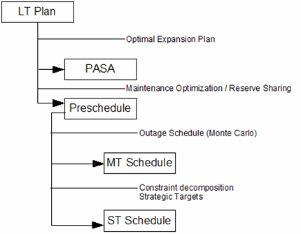 Figure 1: Integration of simulation phases
3.6. Capacity Expansion Planning
Capacity expansion is implemented via the LT Plan simulation phase.
The purpose of the LT Plan is then to solve the capacity expansion
problem over the planning horizon: typically expected to be in the
range of 10 to 30 years, though any horizon is possible. LT Plan
appropriately deals with discounting and end-year effects.
The following types of expansion/ retirement and features are
supported:
- Building new generating plant
- Retiring existing generating plant
- Multi-stage projects
- Building or retiring AC and DC transmission lines
- Multi-stage transmission projects
- Expanding the capacity on existing transmission interfaces
- Taking up new physical generation contracts
- Taking up new physical load contracts
- Developing gas fields and pipelines
- Developing gas storage
- Co-optimizing electric and gas expansion decisions
- Deterministic or stochastic optimization
Refer to the article Long Term Planning for more details.
3.7. Capacity Adequacy and Maintenance Planning
These aspects are handled by the PASA
simulation phase
PASA supports three outage types:
Discrete maintenance
Maintenance events that are known in advance
Distributed maintenance
Maintenance events generated by the simulator
Forced outage
Unexpected outages generated by the simulator
NOTE:Transmission Node objects can also be added/ removed dynamically during the simulation with the units property.
Discrete maintenanceDiscrete maintenance events represents planned outages, such as major thermal boiler repairs, or regular outages, whose timing and during are known. Data defining these outages is defined as properties for Generator objects with the units out property (and similarly for line and gas pipeline.
Distributed maintenanceDistributed maintenance represents regular outages that are part of the normal maintenance schedule for the unit but for which the timing is not known a priori. PASA can time these outages; taking into account discrete maintenance by balancing regional capacity reserves over an annual timeframe.
Forced outageForced outages are those random outages that occur during the normal operation of the generating units or transmission lines. The simulator will generate random outages according to the properties Generator forced outage rate and mean time to repair (and similarly for line and gas pipeline).
Outage durationPLEXOS supports the definition of outage duration functions for each generator or line in any of these alternative distributions: Fixed duration, uniform, triangular, exponential, weibull, lognormal, SEV, LEV.
Outage severityOutages may be full e.g. whole generating unit outages are partial e.g. interconnector derating or partial thermal derating. Please refer to the article Maintenance Scheduling for more information.
Maintenance timingPASA optimizes the timing of maintenance events such that regional/zonal capacity reserves are levelised accounting for the sharing of capacity between regions/zones via the transmission network.
Reliability statisticsPASA calculates the standard reliability statistics such as LOLP, LOLE, EENS and EDNS.
Sampling and convergencePASA supports both standard Monte Carlo and Convergent Monte Carlo techniques. The latter is used to reduce the number of samples of random outages modelled to obtain a level of convergence.
3.8. Medium- term scheduling and simulation
MT Schedule can be executed stand-alone or run in concert with the other models as in Figure 1. In stand-alone mode MT Schedule can be used to give fast for medium to long-term studies. When run as a component its results are automatically linked to the ST Schedule so that the impact of constraints such as energy limits and storage targets can be correctly accounted for in the short-term schedule.
The MT Schedule handles all user-defined constraints including those that span several weeks, moths or years. This might include:- Fuel off-take commitments e.g. gas take-or-pay contracts
- Energy limits
- Long-term storage management taking into account inflow uncertainty
- Emission quota
Each constraint is optimized over its original timeframe and the MT Schedule to ST Schedule Bridge algorithm converts the solution obtained, e.g. a storage trajectory, to targets or allocations for use in the shorter step of ST Schedule.
ChronologyMTSchedule offers a number of
options for reducing the temporal detail. This is controlled by the Chronology.
Under "Partial" chronology each day, week, or month is defined by set
of load (or price) duration curves (LDC) each with a number of blocks.
The blocks are designed with more details in peak and off-peak load
times and less in average load conditions, thus preserving some of the
original volatility, although there a multiple slicing methods
available.
The simulator schedules generation to meet the load and/or clear
offers and bids inside these discrete blocks. All system constraints
are applied, except those that deal with generator unit commitment and
other intertemporal constraints that imply a chronological
relationship between intervals. Chronological is preserved between LDC
though i.e. between day or week or month depending on the settings for
MT Schedule.
The LDC approach maintains consistency of inter-regional load
profiles, ensuring that coincident peaks are captured.
Under "Fitted" or "Sampled" chronology options, unit commitment and
other intertemporal details such as ramp constraints are preserved
giving a more accurate simulation at the cost of additional
computation time. .
MT Schedule can model competitive behaviour of portfolios over the medium term. This can be 'simply' recovery of fixed costs (LRMC), or more sophisticated game-theoretic behaviours like Nash-Cournot competition.
3.9. Short-term Scheduling and Simulation
ST Schedule is a full
chronological model i.e. it solves the actual market interval time
steps (of any length e.g. 5 minutes, half-hour, or hour) over a
horizon from one interval to many years.
Some example uses of ST Schedule
are:
- A market-clearing dispatch and pricing problem based on generator offers and load bids
- A large scale transmission study
- A traditional thermal unit commitment and coordination problem
- Portfolio optimization
- Stochastic unit commitment
ST Schedule generally executes in steps spanning a number of days or weeks, and receives information from MT Schedule that allows it to correctly handle long-run constraints in this shorter time frame.
3.10. Stochastic Variables
PLEXOS provides comprehensive stochastic modelling and optimization capabilities and this applies across all simulation phases from LT Plan through to ST Schedule. There are two distinct types of stochastic inputs:
- Outages (either planned or unplanned)
- random variables (either user-defined samples or synthetic samples generated by the simulator)
Outage-related input properties are described in the Forced outage
and maintenance section.
The number of outages patterns generated is controlled by the
Stochastic Outage Pattern Count setting. Each simulation phase has a
Stochastic Method setting that controls how these multiple patterns
are simulated. Setting this control to "Independent Samples" (either
sequential or parallel variations) invokes the Monte Carlo simulation
mode, whereby the simulation is repeated for each outage pattern.
Results are produced for each 'sample' and various settings of the
Report object control the extend of reporting for the samples and
statistics.
The Variable class is a powerful
tool for creating randomized sample data for a wide range of inputs.
In fact, practically any input property can be randomized through the
Variable class. Some commonly used examples are load, wind, solar,
hydro inflows, fuel and electric prices. A Variable object can be used
to read either user-defined sample data or to automatically generate
sample data during the simulation based on user-defined parameters of
the probability distribution.
The number of samples simulated is controlled by the Stochastic
Risk Sample Count
setting.
The stochastic mode by simulation phase and reporting of samples and
statistics for simulation outputs is controlled in the same manner as
for a multiple outage pattern run.
The Stochastic Method setting, which is found on each simulation phase separately, includes a stochastic optimization mode called "Scenario-wise Decomposition". This mode is different from Monte Carlo simulation in that it overcomes the perfect foresight assumption of running independent samples and seeks a set of non-anticipative decisions for user-identified decisions such as unit commitment or hydro release policies. See the article Unit Commitment for more details.
3.11. Models of Imperfect Competition
Advanced features are available to model imperfect competition and thus produce market price outcomes that reflect real market behaviour.
Company Class of ObjectsThe concept of ownership is supported of generation, purchaser, physical, financial and fuel contracts, market transactions and transmission assets through the Company class of objects.
Contract SettlementDifference payments are calculated on contracts for differences (CFD) and other contracts such as one-ways. Settlement residues (transmission congestion rents) are also reported.
Allocation and Recovery of Fixed CostsCompany class represents common ownership, and hence a model of the underlying market structure and level of competitiveness. The Company article provides references to the oligopoly modelling features, which can be used to set generator pricing options, and control recovery of fixed costs, and perform market power analysis.
3.12 Solver engines
PLEXOS is tightly integrated with a number of commercial and academic solvers including the best and fastest commercial mathematical programming solvers available:
- CPLEX
- Gurobi (Preferred)
- MOSEK
When you license PLEXOS you can choose any or all of these solvers as the engine that PLEXOS uses to solve the linear, quadratic, and mixed integer programming problems representing the simulation task.
3.13. Output
Detailed outputs is derived from the solution of the various simulation phases. All output properties are described in the Class Reference section, and the report options under the Report topic.
3.14. Program Architecture
The software architecture of PLEXOS is illustrated in Figure 2:
- Data are input to a database via the PLEXOS graphical user interface.
- Database entries may refer to text files for data series e.g. load forecasts.
- The simulation engine reads the database, extracting the data selected for the current simulation, executes, and produces one or more solution databases and/or text files.
- Solution databases can be queried/browsed via the GUI or automatically using the COM or .NET libraries.
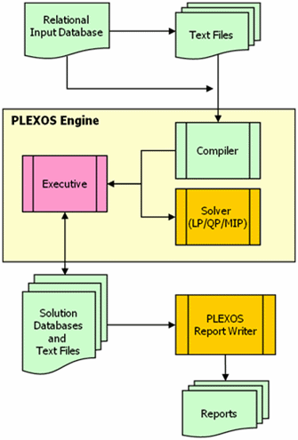 Figure 2:Program Architecture
The simulation engine has the layout shown in Figure 3: the key points are:
- Written entirely in the Microsoft .NET framework;
- It seamlessly integrates: data collection; mathematical program formulation and solution via the integrated solvers; and solution retrieval;
- The unique "AMMO" component inside the engine implements the dynamic formulation engine.
- Formulation adapts to problem data;
- Problem size is minimized;
- Execution speed is maximized;
- Single code base supports multiple applications; and
- No preset limits on problem size; or simulation functionality.
AMMO performs a similar role in PLEXOS as other mathematical languages such as AIMMS, AMPL, or GAMS but is written exclusively for PLEXOS.
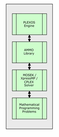 Figure 3: PLEXOS Engine Layout
3.15. Object Model
As described earlier, PLEXOS is constructed around an Object Model.
That model defines a set of classes, a hierarchy, and rules about how
objects interact and relate to each other. Each input file implements
the Object Model.
The model is based around three basic elements:
- Object
- Memberships (also called "relationships"); and
- Properties (the data)
All features are accessible through this object model. The PLEXOS interface makes it easy to navigate and edit data in the Object Model.
4. Load and Transmission
This chapter describes how load and transmission is represented. It
gives a brief introduction to the Region,
Zone, Node,
and Line classes. We assume that loads
are entered as fixed quantities: for loading bidding refer to the Purchaser class.
You can think of Region objects as representing transmission "areas".
Zone objects can be either subsets or supersets of Region, and load
can be defined at either the Region or Zone level or both.
Node is the connection point for objects such as Generator and no
matter how load is defined it will be distributed to Node objects in
the simulation.
4.1. Load
Loads can be defined either in aggregate on Region
and/or Zone objects, or at individual
network nodes using Node objects.
When modelling the electric system, your input file must define at
least one object. If this is all your
model requires then no further data are needed. Implicitly the
simulator will include a Node object and place it in that Region so
that all load defined on the Region is occur at the Node. This feature
is for the convenience for users that do not wish to create a
transmission network representation.
If you need to model more than one Region or Node you will need to
enable the Node class via Configuration. Once the Node class is
enabled you associate each object with a Region via the Node Region
membership.
If you are modelling only regional level transmission (with no
transmission detail inside the regions) then create one Node per
Region and define the load on the Region objects.
Inside any Region you can create multiple nodes to model an AC network
in detail. Each Node must be associated only with one Region using the
Node Region membership. Nodes may also have a Zone membership. The
load can then be defined on the Region and/or Zone and distributed to
the nodes using the Node Load
Participation Factor property; or alternatively you can define
the load directly on the nodes using Node Load.
You may also associate a Zone with a Region via the Zone Region
membership and distribute the Region Load with the Zone Load
Participation Factor.
Regions are also used to define areas in which maintenance outages
should be "optimized" in order to equalize reserves. They also affect
certain unit commitment methods such as the "Rounded Relaxation".
The relationship between the system being modelled and the Region objects in a PLEXOS file depends on the structure of the market. For example, in modelling the:
- Australian NEM, a region represents each state;
- New Zealand NZEM each island is a region;
- Californian market each transmission area is a region;
- European continent each country is a region.
To build the required representation, first create the Region and
Node objects. Then for each Node, add the Region it belongs in to its
Region collection you can create the complement instead by adding the
Node to the Nodes collection. This relationship means that the Node
will acquire load information from that Region (and vice versa), and
be included in that region's summary of load, generation, price, etc.
Regions need to report an energy price from the market. In systems
with multiple nodes per region the default is to report a
load-weighted average price. This behaviour can be changed using the
Design class of objects.
Load data are usually read from text files, the required format for
which is described in the article Text File Formats. The Region or
Node Load property then points to that text file via the Data File
field in the dynamic property grid. The file must contain a header
row. The most common format to use is referred to as "Periods in
Columns" format:
- The first three columns set the year, month, and a day;
- The remaining columns hold load figures for each interval of the day;
Each text file contains the interval-by-interval loads for one region
only unless you add a Name field as the first field in the file
containing the names of the Region objects the load pertains to.
Regions are not required to define load if there is no load in a
particular region. Refer to the Text File Formats article for
information on other file formats.
Example 1: Load values are read from a CSV format file
| Property | Value | Unit | Data File |
|---|---|---|---|
| Load | 0 | - | North.csv |
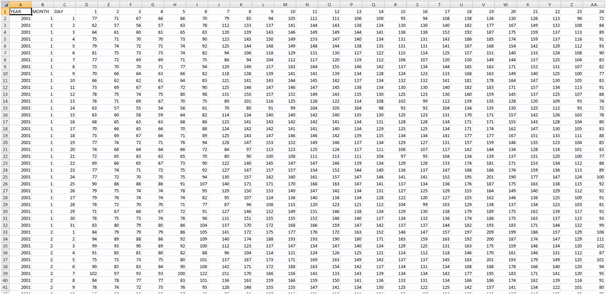 Figure 4: Example CSV file
Example 2: Loads are defined using a pattern and scaling factors
| Property | Value | Unit | Date From | Timeslice |
|---|---|---|---|---|
| Load | 90 | - | - | H01 |
| Load | 74,47 | - | - | H02 |
| Load | 60 | - | - | H03 |
| Load | 47.57 | - | - | H04 |
| Load | 38.04 | - | - | H05 |
| Load | 32.04 | - | - | H06 |
| Load | 30 | - | - | H07 |
| Load | 32.04 | - | - | H08 |
| Load | 38.04 | - | - | H09 |
| Load | 47.57 | - | - | H10 |
| Load | 60 | - | - | H11 |
| Load | 74.47 | - | - | H12 |
| Load | 90 | - | - | H13 |
| Load | 105.53 | - | - | H14 |
| Load | 120 | - | - | H15 |
| Load | 132.43 | - | - | H16 |
| Load | 141.96 | - | - | H17 |
| Load | 147.96 | - | - | H18 |
| Load | 150 | - | - | H19 |
| Load | 147.96 | - | - | H20 |
| Load | 141.96 | - | - | H21 |
| Load | 132.43 | - | - | H22 |
| Load | 120 | - | - | H23 |
| Load | 105.53 | - | - | H24 |
| Load Scalar | 1 | - | - | - |
| Load Scalar | 1.1 | - | 1/01/2010 | - |
| Load Scalar | 1.21 | - | 1/01/2011 | - |
| Load Scalar | 1.33 | - | 1/01/2012 | - |
It is important that the load data are consistent with the generation and load representation. There are two settings that affect the load formulation:
- If the load entered is 'sent out' (net of station auxiliary loads)then you should set the attribute Region Load Metering Point = "Sent out"; otherwise accept the default of "Generator Terminal".
- If the input load includes transmission losses that will also be modelled by PLEXOS you should set Region Load Includes Losses = True; otherwise accept the default of False.
For example, in the Australian NEM, forecasts of load are made of the total consumption in the state with imports and exports measured at region boundaries (gross), but energy forecasts are made on a 'sent-out' (net) basis. You should be very careful about what figures you are using and make sure your input and options match each other.
Distribution of Load in a Multi-node RegionThe proportion of the total regional load that is placed on each node is based on Node [Load Participation Factor]. The default value of this property is:
- One if the region has only one node;
- Zero if the region has more than one node.
Therefore in a multi-node region, it is important to set these factors at each load node; but you do not need to set it for non-load nodes.
Creating Input Load ProfilesRefer to the article Load Forecasting
4.2. Transmission Network
The transmission network is defined using Node and Line objects (and
for more advanced use Transformer, Phase Shifter objects). A Node
represents a busbar in the transmission network, and a Line can
represent any type of transmission line (AC or DC). Because Lines are
an abstract object they can represent a single line or notional
interconnector alike.
Lines require two memberships: a Node in their Node From collection
and one in their Node To collection: the nodes cannot be the same. An
example is given in Figure 5. Here the Line "DE-NL" flows from Node
"DE CP" to Node "NL CP".
The reference direction for the line defines what is meant by positive
versus negative flows. In this example if the line has a positive flow
it is flowing from "DE CP" to "NL CP". The limit in the reference
direction is set by the Line Max Flow property, while the limit in the
counter reference-direction is set by Min Flow as in Table 4. Note
carefully the sign of the minimum flow limits (negative by
convention), and also that you do not need to define Min Flow as it
will default to the negative of Max Flow.
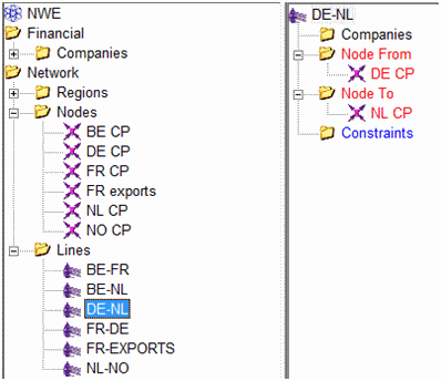 Figure 5: Example Line Configuration
Table 4: Line limits
| Name | Property | Value | Unit |
|---|---|---|---|
| DE-NL | Max Flow | 2100 | MW |
| DE-NL | Max Flow | -3000 | MW |
The linearized DC-OPF method that computes transmission AC network
flows fundamentally assumes resistance is zero and all voltages are 1
pu. However the formulation used here can incorporate losses as an
extension of the standard DC-OPF method. In addition, losses can
always be modelled on DC lines and when approximating the network as a
transportation model.
You have three options for considering losses in the transmission
network and these are (in order of complexity/accuracy):
- Ignore losses in dispatch and pricing and simply report the losses that would occur. This is achieved by defining the loss parameters on Line objects (as below) and setting Transmission Losses Enabled = False.
- Model only the marginal (pricing) effect of losses by defining the transmission loss factors (TLF) through the Generator Marginal Loss Factor property.
- Model losses in dispatch and pricing with Transmission Loss Enabled = True.
Line losses can be specified in one of two ways:
- Using the Line Resistance property; or
- Defining a custom quadratic function: using the Loss Base, Loss Incr, and Loss Incr 2 properties (reference direction), and (optionally) Loss Base Back, Loss Incr Back, and Loss Incr 2 Back properties (counter reference direction).
Losses on Transformer are defined with the Resistance property.
NoteThe default MVA Base for input of Line Resistance is 100 MVA. There are a number of algorithmic options for handling losses and these are described in the article Loss Modelling. The default settings work well for regional modelling.
Optimal Power FlowAs mentioned above, optimal power flows in the AC network can be
computed using a linearized DC load flow model with integrated losses.
The OPF is co-optimized with unit commitment and dispatch.
A transmission line is considered AC if it defines Line Reactance (or
alternatively Susceptance). Any number of disjoint AC networks can be
modelled and the OPF is computed in each. Lines and nodes going in/out
of service mid-simulation either for planned or random outages can
also be handled.
The Transmission object includes many controls for transmission
modelling. Several of these options refer to the voltage transmission
elements. Thus it is useful to set Node Voltage to identify the
voltage level of nodes and connecting lines.
For the linearized DC-OPF there are two distinct formulations
available, and these are described in the articles Linearized DC OPF
and Loss Modelling.
Any number of contingencies can be defined. The simplest way is to set Transmission N-1 Contingency Voltage Threshold and n-1 will be modelled automatically. Finer control and multi-element contingencies can be defined with Contingency objects.
5. Generators
This chapter introduces the Generator class. A Generator object may be used to represent any of the following in any combination:
- A market participant that offers generation to the market
- A single generating unit
- A generating station with multiple units
- A thermal generator that uses various fuels
- A component of a combined-cycle (CCGT) plant
- A combined heat-and-power (CHP) plant
- A hydro generator that draws water from a storage, passing it to another storage and/ or pumps water from one storage to another
- A wind generator
- Other renewables such as solar
- A controllable load (so-called 'anti-generator')
Note that the purchaser class mirrors much of the generator class functionality but for dispatchable load rather than generation.
5.1. Creating a Generator
Generator objects are created in the normal way: see help article User Interface Guide. Like any object in a collection they must have unique names no more than 50 characters in length. The optional Category field can be used to sort the objects into some order other than the default alphabetical order. For example, it might be convenient to sort generators by location and/or type (baseload, intermediate, hydro, and peaking). The pop-up menu Categorize command is used to define these categories.
Units and CapacityThe Generator Units and Max Capacity properties must be defined
before the generator can be considered available i.e. the generator is
available when the Units property is set to a non-zero value and there
is some non-zero capacity. The Max Capacity property defines the size
of the units in megawatts.
If the generator is not installed until after the start of the
planning horizon, it is sufficient to set the Date From field in the
generators Units property as in the following example. It will be
assumed prior to this that zero units are installed.
Example: Generator Units and Max Capacity properties
| Property | Value | Units | Date From |
|---|---|---|---|
| Units | 1 | - | 1/01/2012 |
| Max Capacity | 150 | MW | - |
As with any property the Units property can be labelled with a
Scenario allowing the evaluation of different generator entry
scenarios in different Model runs.
If units are decommissioned during the planning horizon, simply add
another Units entry with the appropriate date as in the following
example.
Example: Decommissioning units
| Property | Value | Units | Date From |
|---|---|---|---|
| Units | 1 | - | - |
| Units | 0 | - | 1-May-04 |
Multi-unit stations are defined exactly like single units, except that the Units property will be set to a value greater that one. The units are assumed to have identical characteristics such as maximum and minimum capacity, heat rate, outage and maintenance rates, etc. In dispatch, all available units are treated identically but may be committed individually. Committed units, however, are assumed to share the total station load evenly between them.
5.2. Generator Injection Point
Generators are required to have a Generator Nodes membership (though this is implied if the Node class is disabled). This membership indicates which transmission node the generator injects at. Generators can inject at multiple nodes simultaneously (useful for modelling hydro plant that represent an aggregated chain of plant). In this case you should set the property Generator Nodes Generation Participation Factor to distribute the generation correctly between the multiple nodes.
5.3. Station Auxiliaries and Loss Factors
The Max Capacity value is always the gross generation figure. Auxiliary loads are defined using the properties Aux Fixed, Aux Base, and Aux Incr i.e. they define how the units at the station use power when installed and when operating:
- Aux Fixed is the megawatt load drawn by each installed unit at the station. This load is independent of the commit status or load of the unit
- Aux Base is the auxiliary loss of a unit at minimum load in MW
- Aux Incr is the auxiliary load per unit of load (MW/MW).
Typically the Aux Incr property is used to convert generator terminal
(gross) unit ratings to sent-out (net) figures as in the following
example, in which the generator is defined with 7% auxiliary losses.
Example: Generator auxiliary losses
| Property | Value | Units |
|---|---|---|
| Units | 4 | - |
| Max Capacity | 660 | MW |
| Aux Incr | 7 | % |
See the section Load above regarding the interpretation of the input load figures and make sure that your generator auxiliary loss definition is consistent with the load settings.
5.4. Fuel Use and Constraints
Generators consume fuel according to their unit heat rate function
expressed in units of GJ/MWh (metric model) or BTU/kWh (Imperial US
model). In some modelling situations however, recording fuel use is
unnecessary e.g. when using the simulator as an offer and bid clearing
engine or for renewable resources that do not consume any fuels per
se. In this situation fuel use is assumed zero, and the cost
production is determined purely from generator offers or by the
variable cost of maintenance (the Generator VO&M Charge property).
In most situations though, the cost of production must be calculated
by multiplying the fuel price by the unit heat rate. Three mechanisms
are provided for setting the fuel price for a generator and multiple
input schemes for specifying the heat rate function of a unit.
The simplest way to set the fuel price on a generator is use the Generator Fuel Price property. The advantage of this technique is that it allows there to be a different fuel price on each Generator; the disadvantage is that it may involve repeating information across several generators that use the same fuel.
Fuel ObjectsThe more common method is to create Fuel objects and associate generators with them using the Generator Fuels] membership. This way you can:
- Have multiple generators use the same fuel
- Apply constraints on fuel usage
- Model fuel-based emissions
If the cost of the fuel varies according to the location of the generator use the Generator Fuels Transport Charge property as a adder to the 'base' Fuel Price.
Gas Network ConnectionConnecting a Generator to a Gas Node and simultaneously associating the Generator with a Fuel enables the supply of 'gas' from the gas network to the Generator. The cost of gas is then set by the combination of gas production costs and any charges on the Fuel.
Multi-fueled UnitsGenerators might be fueled by more than one fuel type e.g. a primary
(cheap but limited) and a secondary fuel, or connected to the gas
network as well as supplied by another back-up fuel such as liquid
fuel. Fuel objects must be used to model this situation. Any number of
Fuel objects may be added to the Fuels collection of a Generator.
There is no distinction made in the model input between primary and
secondary or other fuels. These fuels are used in order of cheapest
first, taking into account any constraints on supply of the fuels.
The cheapest fuel will always be used unless a constraint is placed on
the offtake of that fuel. Offtake constraints can be defined using the
many built-in constraints such as Fuel Max Offtake or for more complex
forms using the Constraint class: see section Generic Constraints.
Switches between fuels are done automatically according to the
implicit values of each available fuel i.e. more expensive fuels will
be used at peak times. These fuel trade-offs are fully optimized
inside the mathematical formulation resulting in the most efficient
possible fuel use.
When the ratios of fuel mixing are fixed, use the Generator Fuels
Ratio property to define the fixed ratios. You can also define a
penalty for violating the fuel mixing constraints; which is useful
when the defined ratios are 'desired' but might be infeasible due to
other constraints. Other properties are available to set minimum and
maximums input and ratios.
A Generator object can be defined as using a fuel (or fuels) for
starting that are different to its fuels for generating. Adding Fuel
objects to the Generator Start Fuels collection establishes this
relationship. The amount of fuel used to start the unit is controlled
by the property Generator Start Fuels Offtake at Start defined on the
membership.
The fuel used to start a unit combines with the Generator Start Cost
property to set the total cost of starting a unit.
When using multiple bands of Start Cost to represent hot, warm, cold
starts you can also use multiple bands on Generator Start Fuels
Offtake at Start.
For hourly resolution modelling it is usually adequate to assume that generators start up and reach Min Stable Level within a dispatch period. For sub-hourly modelling in particular, this assumption might not be valid. In this case use the Generator Generator.Run Up Rate and/or Run Down Rate. More complex forms of these constraints defined with the Start Profile and Shutdown Profile properties.
5.5. Unit Heat Rate
Definition of the unit heat rate function for thermal generators is supported using one of a number of formats including:
- Constant heat rate using Heat Rate or Heat Rate Incr
- Incremental heat rates using Heat Rate Incr and Load Pointin multiple bands
- Average heat rates using Heat Rate and Load Point in multiple bands
- Polynomial function using Heat Rate Base, Heat Rate Incr, Heat Rate Incr 2 and Heat Rate Incr 3
These properties are described in detail in the article Heat Rate
Modelling. In the following we describe the common usage of these
properties.
The Generator property Heat Rate determines the amount of fuel used
per megawatt of generator load i.e. Fuel Offtake = Heat Rate ×
Generation. In the simplest case, where only the Heat Rate property is
defined, a single heat rate will apply across the entire range of
generator loads.
Example: Generator with constant heat-rate (metric)
| Property | Value | Units |
|---|---|---|
| Units | 4 | - |
| Max Capacity | 660 | MW |
| Fuel Price | 1.16 | $/GJ |
| Heat Rate | 9.42 | GJ/MWh |
Example: Generator with constant heat-rate (Imperial US)
| Property | Value | Units |
|---|---|---|
| Units | 4 | - |
| Max Capacity | 660 | MW |
| Fuel Price | 1.16 | $/MMBTU |
| Heat Rate | 9420 | BTU/kWh |
Heat rate generally varies across a unit's operating range. In this
case it is convenient to specify the heat rate at several points. This
is done using the Load Point property in combination with Heat Rate
(or Heat Rate Incr for incremental rates) as in the following example.
Example: Multi-point heat rate function using average rates (metric)
| Property | Value | Units | Band |
|---|---|---|---|
| Units | 4 | - | 1 |
| Max Capacity | 660 | MW | 1 |
| Min Stable Level | 264 | MW | 1 |
| Fuel Price | 1.16 | GJ/MWh | 1 |
| Load Point | 264 | MW | 1 |
| Load Point | 660 | MW | 2 |
| Heat Rate | 11 | GJ/MWh | 1 |
| Heat Rate | 9.42 | GJ/MWh | 2 |
The Band is used to match the load points with the heat rates. The
heat points must be in order or an error will be reported. Note
further that the load point values need not match the Min Stable Level
and Max Capacity.
The previous two-band examples result in a linear heat function. A
third band can be added, which will produce a quadratic function. Any
number of points can be specified, and the simulator uses the points
to fit a order-3 polynomial to the implied fuel use function, which is
then in turn converted into a piece-wise linear incremental heat rate
function with the number of tranches determined by Max Heat Rate
Tranches.
If your data is for incremental heat rates, rather than average, then
use the Heat Rate Incr property instead of Heat Rate.
An alternative to the load point/heat-rate method is the specification
of the properties Heat Rate Base, Heat Rate Incr, Heat Rate Incr 2 and
Heat Rate Incr 3. These parameters describe a order-3 polynomial
function directly.
By default the data provided to define the heat function are used to fit a order-3 polynomial and then a piece-wise linear approximation with Max Heat Rate Tranches number of tranches. You can overrides this behaviour and force the simulator to use your input curve verbatim by defining more load points than Max Heat Rate Tranches.
Heat Rate by FuelThe heat rate function may vary by fuel type used. Fuel-specific heat rate functions can be defined on the properties of the Fuel object inside the Generator Fuels collection. Any settings here override the fuel use function defined on the Generator.
ConvexityThe marginal heat rate function should be monotonically non-decreasing unless you set the Production Heat Rate Error Method = "Allow Non-convex". Refer to the article Heat Rate Modelling for details on how the simulator deals with non-convex functions.
Short-run Marginal CostThe short-run marginal cost of generation at a particular megawatt
level is calculated as the fuel price (as defined above) combined with
the heat rate function and VO&M Charge i.e.:
SRMC = Fuel
Price × Heat Rate Incr
+ VO&M Charge
Where Heat Rate Incr is derived from the polynomial fit to heat
function.
5.6. Offers
Offers for generation can be used to define capacity and price on
their own or to override the short-run marginal cost (SRMC) pricing.
Generator offers do not affect the calculated cost of generation, only
the prices and quantities offered to the energy market.
Generator offer quantities are assumed to be generator-terminal
(gross) values while offer prices are sent-out (net) values.
The properties Offer Quantity and Offer Price define a set of
multi-band offers for a generator. Note the following:
- Offer Quantity is by default incremental but can be changed to cumulative (like Load Point with the setting Generator Offer Quantity Format
- There is no limit to the number of offer bands that can be input but you should use the Configuration form to set the number of bands you want to use
- By default the offer bands are cleared lowest to highest in price unless you set the Generator attribute Offers Must Clear in Order
- Offers can vary over time using the Date From, Date To, and Timeslice fields, or read from files using the Data File field
- Generation offer quantities never override the Max Capacity but if the total quantity offered is less than Min Stable Level that constraint is relaxed to allow generation according to the offers.
Example: Defining a multi-band Offer
| Property | Value | Units | Band | Timeslice |
|---|---|---|---|---|
| Offer Quantity | 140 | MW | 1 | - |
| Offer Quantity | 35 | MW | 2 | M1-3,12 |
| Offer Quantity | 50 | MW | 2 | M4-11 |
| Offer Price | 0 | $/MWh | 1 | - |
| Offer Price | 45 | $/MWh | 2 | - |
The number of bands that have been defined on a Generator is allowed to change across the horizon, with inactive bands assumed to have a zero Offer Quantity by default.
Offers on Multi-fueled UnitsOn multi-fueled units, the generation offer applies to all fuels unless you define the individual offers using Generator Fuels Offer Quantity and Offer Price.
No Load CostFor electric markets with centralized unit commitment (e.g. Ireland) additional offer data can be defined. Offer No Load Cost is a cost incurred for any hour that a unit is committed.
Balancing market offersIn a balancing market, offers are 'centred' around a base value and the offer is divided in to increment and decrement parts being offers to increase generation from the base and bids to decrease respectively. See the article Balancing Markets for details.
Pumped Storage BidsBids can be defined for pumped storage units with the properties Pump Bid Quantity and Pump Bid Price.
5.7. Mark-up
A mark-up is a price for generation above marginal cost. Mark-ups
might be required to recover fixed costs or semi-fixed costs like
Start Cost and no-load cost (see the article Heat Rate Modeling for a
definition). The Competition setting No Load Cost Mark-up
automatically adds a mark-up that will recover no-load cost.
For manually defined mark-ups, the property Generator Mark-up is the
absolute amount that the generation of the unit is marked up above
marginal cost. If you prefer a relative mark-up use the property Bid
Cost Mark-up and optionally additional Mark-up i.e. the two properties
can be used together.
Both properties can be multi-band when used in conjunction with the
Load Point properties as in this example:
Example:Mark-up Properties
| Property | Value | Units | Band |
|---|---|---|---|
| Bid Cost Markup | 0 | % | 1 |
| Bid Cost Markup | 20 | % | 2 |
| Bid Cost Markup | 50 | % | 3 |
| Bid Cost Markup | 120 | % | 4 |
| Load Point | 40 | MW | 1 |
| Load Point | 70 | MW | 2 |
| Load Point | 90 | MW | 3 |
| Load Point | 100 | MW | 4 |
5.8. Unit Commitment
In chronological simulation phases (any of LT Plan, MT Schedule and
ST Schedule depending on settings) generator unit commitment and
economic dispatch (UCED) is optimized using mixed-integer programming.
Unit commitment decisions are optimized across each step of the
simulation, where the step size is configurable to any length
(minutes, hours, days, weeks) and additional look-ahead can be
specified. Deterministic, Monte Carlo simulation and stochastic unit
commitment functions are available. See the article Unit Commitment
for details.
The following table describes the common generator properties related
to unit commitment and gives an indication of the difficulty of
modelling them in terms of computation time and problem size. You
should use this as a guide when determining the most appropriate data
for your Generator objects in terms of accuracy versus computation
time.
Table 5: Unit commitment related properties
| Property | Description | Computational Implications |
|---|---|---|
| Min Stable Level | The minimum generation level when the unit is committed | Adds only one additional constraint per generator/period to the formulation. Generally easy for the solver to optimize, unless MSL is a very high proportion of capacity. |
| Min Up Time | The minimum number of hours that a unit must run for once it has been started | Adds multiple variables and constraints to the formulation. The longer the minimum up time, the more terms are added, so long times can produce a large formulation. These limits are relatively difficult for the solver. |
| Min Down Time | The minimum number of hours that a unit must be down after it has been shutdown | As above for minimum up time |
| Start Cost | The cost of starting up a unit | Start cost adds variables and constraints to the formulation. If you define multiple start costs as a function of the number of hours a unit has been down (cold, warm, hot, etc) then additional integer variables are required in the formulation and this can be difficult for the solver to optimize. |
| Run up Rate or Start Profile | A specific regime of megawatts steps that a unit must run through as it starts up | Adds constraints to the formulation. Start profile is no more difficult than start cost for the solver. |
| Run Down Rate or Shutdown Profile | A specific regime of megawatts steps that a unit must run through as it shuts down | As above for [Start Profile] |
By default only the linear relaxation of the unit commitment problem
is solved. In the linear relaxation the constraints on minimum stable
level, and minimum up and down times will not necessarily be obeyed:
because they represent an integer not linear decisions. Start costs
will influence the dispatch but not in the same way as they would if
the problem were solved as a mixed integer program.
Use the Production Unit Commitment Optimality setting to switch
between linear and integer modes. You can also choose this setting by
Generator object using the Generator Unit Commitment Optimality
property: thus you can decide which generators will be modelled with
integer variables and which will remain linear.
Performance of the mixed integer solver is very much a
problem-specific characteristic. You should experiment with solving a
short horizon, determining by experimentation the best combination of
options to use, before attempting to solve the complete horizon.
The Performance class offers a number of tuning parameters for the mixed integer solver and solver-specific settings can be made through Hidden Parameters.
Rounded RelaxationThe linear relaxation to the unit commitment problem is problematic
not just because the integer type constraints can be violated but also
because the linear start and unit commitment variables can be 'basic'
variables and thus affect the shadow prices. More specifically the
cost of starts and the no-load cost of generation can affect the
market energy prices. In contrast, in an integer solution, the energy
price is based on the marginal cost of thermal generation and does not
include any 'roll in' of start cost or no-load cost.
Thus we always prefer a integer solution, but solving to optimality
using MIP can be time consuming, thus a heuristic unit commitment
method called "Rounded Relaxation" ("RR") is available which solves
with only a small increase in run time over the linear relaxation. See
the article Unit commitment for more details.
If the system being studied is a self-commitment market, generator offers only include Offer Quantity and Offer Price. From the market clearing engine's viewpoint, generating units can switch on and off as required at no cost, and operate at any level. In this type of markets it is the responsibility of the generators' to structure their offers in a manner that is consistent with constraints on unit operation implied by unit commitment: also see below the use of Fixed Load in this context.
Initial Commitment and LoadIn an operational context where the initial commitment state of
generators is known you can input this by setting the properties
Initial Units Generating and Initial Generation. If you are using
minimum up and down constraints you should also define Initial Hours
Up and Initial Hours Down.
Example: Unit is initially 'on' and has been up for six hours
| Property | Value | Units |
|---|---|---|
| Units | 1 | - |
| Max Capacity | 100 | MW |
| Min Up Time | 12 | hrs |
| Min Down Time | 8 | hrs |
| Initial Units Generating | 1 | - |
| Initial Generation | 90 | MW |
| Initial Hours Up | 6 | hrs |
| Initial Hours Down | 0 | hrs |
In the above example it is assumed that, at the start of the horizon, the unit is 'on' and must stay on for another six hours to meet its minimum up time.
5.9. Must-run, Energy and Other Constraints
Several Generator properties are available for modelling restrictions/constraints on the unit commitment and dispatch of generators.
Must-runGenerator Must-Run Units is the number of units at the station that
must be committed. It is free to commit more than this number of
units, and will only commit less if the units are out-of-service.
Example: Unit must run during peak times on weekdays
| Property | Value | Units | Timeslice |
|---|---|---|---|
| Units | 1 | - | - |
| Max Capacity | 100 | MW | - |
| Must-run Units | 1 | - | W1-6,H14-19 |
The Generator property Commit can be used to 'hardwire' generator
unit commitment. Commit specifies the number of units that (if
available) should be committed. The default value of -1 indicates that
the unit commitment should be optimized not pre-determined. Thus
Commit can be used in a pattern to indicate times when a certain
commitment is needed but left at default for other periods and the
simulator will optimize its commitment in those times.
Example: Unit must be committed during weekday peak times and off in
the weekend but freely optimized at other times
| Property | Value | Units | Timeslice |
|---|
Generator Min Load sets a minimum unit load level (subject to unit
availability). Min Load is sometimes used to model the effect of loads
not included in the simulation such as the load implied by heat demand
from a combined heat and power unit.
In self-commitment markets (Australia for example) generators can
define a 'fixed load' profile for a number of hours. This is used to
control the dispatch of the plant by the market during start up and/or
shutdown of large relatively inflexible units. The property Fixed Load
is provided for this purpose. When Fixed Load is non-zero the
generator with dispatch exactly according to those loads, but when
Fixed Load is zero the dispatch is optimized. The behaviour of Fixed
Load can be changed so that zero values are also enforced using the
Generator attribute Fixed Load Method.
When you define a multi-unit generator, both Min Load and Fixed Load apply to the generating station as a whole, not to individual units.
Energy LimitsGenerators can be included in one or more Constraint objects to control their total energy over any period. For example, there may be minimum or maximum energy on a generator over each day, week, month, or year. As a shortcut to using the Constraint class the Generator class includes these energy-related properties:
- Max Energy, Max Energy Hour, Max Energy Day, Max Energy Week, Max Energy Month, Max Energy Year
- MinEnergy/Day/Week/Month/Year
- Max Capacity Factor Day/Week/Month/Year
- Min Capacity Factor Day/Week/Month/Year
Example: A generator subject to minimum load and maximum capacity factor (e.g. simple hydro)
| Property | Value | Units | Timeslice |
|---|---|---|---|
| Units | 1 | - | - |
| Max Capacity | 100 | MW | - |
| Min Load | 20 | MW | M1-5,11-12 |
| Min Load | 40 | MW | M6-10 |
| Max Capacity Factor Month | 40 | % | M1-5.11,12 |
| Max Capacity Factor Month | 75 | % | M6-10 |
The additional property Generator Energy Scalar is provided so that energy limits defined using the above properties can be easily scaled using a factor. This is useful for introducing volatility into the energy limits by applying a Variable to the Energy Scalar.
Rough Running RangesA generator rough running range is a range of load levels that must be avoided. Typically these apply to hydro generators and are load levels that might cause cavitation in the turbines, but you can apply rough running ranges to any Generator. The property Rough Running Point marks the start of a rough running range and Rough Running Range is the length of the range, both properties are in megawatts and can be multi-band to define multiple such ranges.
5.10. Fuel Contracts
The Fuel Contract class provides a set of properties for modelling
constraints and costs associated with fuel contracts. The Fuel
Contract Fuel membership sets up the relationship between the fuel
contract at the fuel it applies to. Applying a fuel contract to a fuel
replaces the need to define a price on that fuel. It is allowed to
apply more than one Fuel Contract to a Fuel, which might then
represent different sources for that fuel.
Fuel Contract availability is set by the property Quantity and its
hour, day, week, month, and year variations. The price is set by the
Fuel Contract Price property. Both Quantity and Price can be
multi-band to represent multiple price tiers for supply of the fuel.
Take-or-pay commitments are modelled using Take-or-Pay Quantity again
with hour, day, week, month, and year versions. Fuel Contract
Take-or-Pay Price sets the penalty price that is paid to avoid the
take-or-pay commitment (per unit of fuel).
5.11. Forced Outage and Maintenance
The article Planned and Random Outages provides a complete guide to
the Monte Carlo simulation of random outages and the method of placing
maintenance outages in time such that capacity reserves are levelised.
Generator Forced Outage Rate sets the expected level of unplanned
outages (annual average) that result in a partial or complete loss of
generating capability for a certain period of time. Likewise
Maintenance Rate for maintenance outages.
The timing of forced outages is random, but repeatable according to
the Model Random Number Seed. Although maintenance timing is guided
close to the optimal placement by PASA the timings are subject to some
randomization i.e. each sample will have a different maintenance
schedule. This is done so that the simulation results across multiple
Monte Carlo samples show meaningful variation and the simulation is
not biased by a single optimized maintenance schedule.
The duration of each outage event can be either constant (by setting
only Mean Time to Repair) or randomized by selecting a distribution
type and appropriate inputs. See Generator Repair Time Distribution.
Partial outages can be modelled. The property Generator Outage Rating
sets the limit of generator load during each outage event.
Multiple outage types (partial, complete, forced, maintenance) can be
defined by using the Band field to separate the definition of
different outages.
Example: Using multiple bands for different outage types
| Property | Value | Units | Band |
|---|---|---|---|
| Units | 1 | - | 1 |
| Max Capacity | 100 | MW | 1 |
| Forced Outage Rate | 7 | % | 1 |
| Mean Time to Repair | 36 | hrs | 1 |
| Forced Outage Rate | 3 | % | 2 |
| Mean Time to Repair | 12 | hrs | 2 |
| Outage Rating | 60 | MW | 2 |
5.12. Fixed Costs
Fixed operations and maintenance costs are input in units of currency
per kilowatt year e.g. $/kW/year. The annual fixed costs are then
based on the installed capacity thus:
FO&M Cost = FO&M
Charge × Units × Max
Capacity × 1000
Fixed O&M charges are important when optimizing capacity
expansion: see the article Long Term
Planning.
If you want to account for the annualized fixed costs of existing
generators you can input those using Equity Charge and Debt Charge.
These charges will add to the total annual fixed costs of the
generator.
The dynamic bidding of generation by companies to recover these fixed
costs can be modelled. The first step in that process is to make a
notional allocation of fixed costs to each interval of the year. The
costs are allocated according to the pool revenue the generator earns
in each interval i.e. the higher the pool revenue in any given
interval, the more fixed costs get allocated to that interval. This
allocation is calculated regardless of whether the cost recovery
algorithm is 'on' or not. That method is enabled via the Competition
Equilibrium Model attribute: see the article LRMC Recovery Algorithm
for more details.
5.13. Combined Cycle Gas Turbine (CCGT)
CCGT are modelled in one of two ways:
- By modelling the individual gas turbines and separate steam turbines each as Generator objects and linking them together using the Generator Heat Input membership
- As a single equivalent Generator object with a complex heat rate function
The first approach is described in the article Combined Cycle. In the second approach the heat rate function of the 'equivalent' single generator can be defined using a multi-band Load Point and Heat Rate Incr set, and the function is allowed to be non-convex (meaning the incremental heat rate can go and up down across the range of operation according to the changes in operation mode of the CCGT).
NoteFor PLEXOS to optimize with non-convex heat rate functions, you need to set the attribute Production Heat Rate Error Method = "Allow Non-convex".
5.14. Combined Heat and Power (CHP)
The CHP modelling feature allows you to:
- Represent the impact of increasing heat load on overall fuel consumption (i.e. on electrical efficiency).
- Model the ability for two or more Generator objects to deliver heat to a single heat demand point, and hence let the model choose which of the generators to use to meet that heat load.
- Model the ability to meet the heat load by heating boilers within a power plant, and to.
- Split the fuel offtake reporting into a power and heat component.
See the article Combined Heat and Power
5.15. Hydro and Pumped Storage
The Generator class models hydro and pumped storage generators. The wide selection of properties available on the Generator class means there are many ways to model hydro as described briefly below and detailed in the Hydro Modelling section starting with the article Hydro Classes.
Hydro as Energy-constrained GeneratorsDefining a 'simple' generator subject to some minimum generation and
maximum energy is the simplest approach to modelling hydro. As
described above, the energy limit can be defined using the various
period type versions of Max Energy
or Max Capacity Factor
Factor, and the run-of-river generation by Min
Load.
Example: Hydro as energy-constrained Generator
| Property | Value | Units | Scenario |
|---|---|---|---|
| Max Energy Week | 2 | GWh | - |
| Max Energy Week | 1.8 | GWh | dry year |
| Max Energy Week | 2.5 | GWh | wet year |
| Min Load | 10 | MW | - |
| Min Load | 6 | MW | dry year |
| Min Load | 13 | MW | wet year |
A hydro generator with storage is defined by adding a Storage object to the Generator Head Storage collection. The Generator Tail Storage collection is used to create cascading networks of storage and generators. See the article Cascading Hydro Networks for more details.
Hydro Generator EfficiencyGenerator Efficiency Base and Efficiency Incr properties sets the
relationship between generation and water throughput, although you may
also use the normal heat rate properties.
It is important to note that the units of storage default to
'potential energy' not volumes of water. To change this see the
article Units of Data.
Example: Hydro efficiency function (metric volume storage model)
| Property | Value | Units | Band |
|---|---|---|---|
| Units | 1 | - | 1 |
| Max Capacity | 60 | MW | 1 |
| Load Point | 20 | MW | 1 |
| Load Point | 40 | MW | 2 |
| Load Point | 60 | MW | 3 |
| Efficiency Base | 58 | cumec | 1 |
| Efficiency Incr | 0.5 | MW/cumec | 1 |
| Efficiency Incr | 0.48 | MW/cumec | 2 |
| Efficiency Incr | 0.42 | MW/cumec | 3 |
For more details on hydro efficiency and head effects see the article Hydro Generator Efficiency and HeadEffects.
Pumped Storage HydroThe properties Pump Efficiency and Pump Load are provided to define pumped storage hydro. Although pumped storage can be included in a hydro cascade it is most commonly modelled as a 'closed loop' system. The system is defined by setting both a Head Storage and Tail Storage for a Generator as in Figure 6 and then defining at least the properties in the example below.
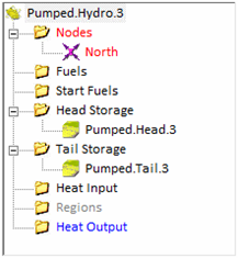 Figure 6:Pumped Storage Membership
For more details see the article Pumped Storage
5.16. Synchronous Condenser Operation
Some generators, particularly hydro, can operate in synchronous condenser mode in order to provide fast spinning reserve. The property Generator Sync Cond Units defines the number of units that can operate in this way. This must be a subset of the Units. Generator Sync Cond Load sets the load drawn while operating in this way. Generator Must-run Sync Cond Units allows you to force a number of units to run in synchronous condenser mode, while Sync Cond VO&M Charge defines the additional operations and maintenance costs.
5.17. Capacity Expansion
A Generator is a candidate for capacity expansion in LT Plan if its Max Units Built property is defined. The overnight build cost is given by Build Cost in $/kW, which can be multi-band to represent a stream of payments leading up to the opening of the plant. The properties WACC and Economic Life can be defined so that the build cost is converted to an annuity.
Example: Thermal plant for capacity expansion
| Property | Value | Units |
|---|---|---|
| Units | 0 | - |
| Max Capacity | 250 | MW |
| Heat Rate | 7.9 | GJ/MWh |
| Max Units Built | 1 | - |
| Build Cost | 1200 | $/KW |
| WACC | 12 | % |
| Economic Life | 25 | years |
Retirement candidates have their Max Units Retired property defined.
Note that Units is always the number of incumbent units, therefore
[Max Units Retired] must be less than or equal to Units plus Max Units
Built.
For more details see the article Long Term
Planning.
6. Reserves/ Ancillary Services
This chapter provides an overview of ancillary services modelling. It is the Reserve class of objects that control this feature.
6.1. Type and Timeframe
Each Reserve object has a type attribute which can be set to one of:
Raise
A spinning up reserve service provided by units online.
Lower
A spinning down reserve service property by units online
Regulation Raise
A regulation up (frequency keeping or load following) service provided by units online separate to their spinning reserve provision
Regulation Lower
As for Regulation Raise but this is the 'down' service
Replacement
Non-spinning reserve provided by units that are not online but that can start quickly
Operational
A combination of Raise and Replacement.
The property Reserve Timeframe is the number of seconds that the
response is required in. This limits the amount of spinning reserves
that generators can provide if they define ramp rate limits and/or
start up times. The Duration property is the length of time that the
reserve must be sustained for, and affects the amount that can be
provided by hydro with storage.
6.2. Reserve Requirement
The amount of the service required is set by the combination of:
- Reserve Min Provision; and optionally
- Reserve Region Load Risk multiplied by the Region Load
The requirement can also be dynamic based on generation and/or
transmission flows. The collection Reserve Generator Contingencies
defines a list of generators, the maximum load (above the Reserve
Cut-off Size) of which sets a reserve requirement. Likewise the
Reserve Line Contingencies collection does the same for line flows,
though you must define either Reserve Line Contingencies Flow Forward
Coefficient or Flow Back Coefficient so it is known what proportion of
reference direction or counter flow is 'at risk'. For generator risk
you can adjust the proportion of generation at risk using the Reserve
Risk Adjustment Factor.
When dynamic risks are included the overall requirement is the maximum
of any one of the contingencies and the Min Provision plus region
demand risk.
You should set the Reserve VoRs property, which is the shortage cost
of reserves, if there is a possibility that the system cannot provide
enough of the service.
6.3. Generator Reserve Provision
The collection Reserve Generators
defines the list of generators that can provide the service. You must
define this set or there will be no generators providing the service.
The effectiveness of the spare capacity provided for reserve can be
adjusted from it default of one-to-one using the property Reserve
Risk Adjustment Factor.
Maximum and minimum reserve provision can be set
generator-by-generator using Reserve Generators Max
Response and Min
Spinning Provision respectively.
Generators can provide spinning 'raise' reserve in four ways:
- By partially loading units
- By running units in synchronous condenser (or "tail-water-depressed" (TWD) mode for hydro units).
- By starting quickly enough to provide a response with the Time frame
- By reducing PumpLoad
Generators can provide 'lower' reserve in two ways:
- By loading units above Min Stable Level
- By increasing Pump Load
The Reserve Generators Max Response and Max Sync Cond Response
properties define how much reserve a unit can provide from each mode
respectively. Max Replacement sets the response limit for replacement
reserves, while Max Pump Response sets the limit for pumped storage.
The property Reserve VO&M Charge sets the additional operations
and maintenance costs associated with providing reserves, and is
charged against all spinning and regulation services.
When a generator is ramping at the time it is called upon to provide
spinning reserve its effectiveness is either reduced or enhanced
depending on the direction of the service and ramp. For example a
generator ramping up is less effective at providing further ramping
for spinning reserve up provision. However, generators can usually
provide a faster rate of ramp for spinning reserve than they their
normal operational ramp rate, thus the property Reserve Generators
Response Ratio is provided, which is equal to the ratio of normal
ramping rate to emergency ramping.
The property Reserve Energy Usage is the proportion of the reserve
provided that will be called upon on average. Generators providing
regulation reserve (in particular) will be called upon regularly. This
implies that fuel (for thermal) and water (for hydro) generators will
be consumed with a certain probability when regulation reserves are
provided. Setting this property means that fuel and hydro energy will
correctly account for reserve provision.
6.4. Reserve Dispatch and Pricing
Reserves are jointly optimized with energy to produce an optimal
dispatch and reserve provision with associated energy and reserve
pricing. Any number of Reserve objects can be defined and
co-optimized.
Reserve can be bought and sold to and from external markets using the
Market class of objects.
6.5. Interruptible Load
There are two types of interruptible Load
- Pumped storage generators in pump mode that can reduce pumping to provide into the spinning up service.
- Loads that can be curtailed to provide spinning up service
Purchaser objects are used to model
interruptible load for the purposes of 'raise' type services (spinning
reserve but not usually regulation reserve). Add Purchaser objects to
the Reserve Purchasers collection to allow those purchasers to provide
interruptible load services.
For pumped storage generators, the Pump Load less the Min Pump Load is
automatically counted as spinning reserve for 'up' services, but you
can set a maximum provision using Reserve Generators Max Pump
Response.
6.6. Offers for reserve provision
The energy and reserve co-optimization results in an endogenous
'price' for the provision of reserve by each generator. There will
naturally be one or more marginal generators for energy and one or
more for each ancillary service, and the market prices for the
ancillary services will naturally emerge from the optimization.
In some markets though, generators and loads can place offer prices on
provision of reserves. The properties Reserve Generators Offer Price,
Offer Quantity are provided for provision of spinning and regulation
and Sync Cond Offer Price for provision of spinning reserve from
synchronous condenser mode, and finally Pump Offer Price for the
provision of pump interruptible load. These offer prices add to the
endogenous price of reserve provision, thus they act as a premium on
the service.
7. Emissions
This chapter provides an overview of the emission and Abatementclasses.
7.1. Emission Objects
The Emission class allows you to define any number of emissions.
Those emissions can be associated with generation and/or fuel use.
Constraints can be placed on emission production across any time
period. Because emission production and any prices and/or constraints
placed on it is fully integrated into the mathematical programming
framework, the generator dispatch and market pricing outcome will
correctly reflect the economic impact of emissions.
You might choose to model the emissions as a function of generation
and/or a function of fuel depending on the type of emission. In
general CO2 is often modelled as a function of generation, whereas SOx
(SO and SO2 by products) is best modelled as a function of fuel used.
NOx (NO and NO2) is often modelled using a combination of generation
and fuel emission properties along with the scaling factor Generator
Fuels Emission Scalar: refer to the help on this property for more
details.
7.2. Fuel Emissions
An Emission object has a Fuels collection, which represents the set of fuels that produce the emission when they are consumed. On this membership, the [Production Rate] property defines the amount of the emission produced per unit of the fuel used. The consumption of the fuel by generators is tracked and the production rate applied to calculate the total emissions produced. The emissions counted will include those from fuel used to start units according to the Generator Start Fuels Offtake at Start property.
7.3. Generator Emissions
An Emission object has a Generators collection, which represents the set of generators that produce the emission either additional to or including those from fuel use. It is on this membership that the property Production Rate is defined, which is the amount of emission produced per megawatt of generation. Note that the property is multi-band meaning that you can combine it with Load Point to define a stepwise marginal emission production function as in the following example:
Example: Generator emissions
| Membership | Property | Value | Units | Band |
|---|---|---|---|---|
| Generator (Big Coal) | Units | 1 | - | 1 |
| Generator (Big Coal) | Max Capacity | 600 | MW | 1 |
| Generator (Big Coal) | Heat Rate | 14 | GJ/MWh | 1 |
| Generator(Big Coal) | Heat Rate | 12 | GJ/MWh | 2 |
| Generator (Big Coal) | Heat Rate | 11 | GJ/MWh | 3 |
| Generator (Big Coal) | Load Point | 200 | MW | 1 |
| Generator (Big Coal) | Load Point | 400 | MW | 2 |
| Generator (Big Coal) | Load Point | 600 | MW | 3 |
| Emission (CO2) Generators (Big Coal) | Max Volume | 30 | kg/MWh | 1 |
| Emission (CO2) Generators (Big Coal) | Max Volume | 35 | kg/MWh | 2 |
| Emission (CO2) Generators (Big Coal) | Max Volume | 40 | kg/MWh | 3 |
that it is not required to provide a multi-band function for
emission production. You can use Load Point multi-band to define your
heat rate function and input a single band for the emission production
rate if preferred.
In addition there can be emissions produced at generator start up and
this is set by the Emission Generators Production at Start property.
7.4. Emission Removal
Generators with emission mitigation technologies can capture some
proportion of their emissions and prevent them from being released.
The property Emission Generators Removal Rate is the proportion
removed. The incremental cost of removal is set by the property
Emission Generators Removal Cost. Thus the net emissions production
for a generator is given by:
(1 - Removal Rate) x Production Rate x Generation
and this is added to by fuel-based emissions:
(1 - Removal Rate) x Production Rate x Heat Rate x Generation
Here the heat rate is used as a placeholder for the average heat rate
in particular generation block.
7.5. Abatement Devices
A more advanced way of modelling emissions abatement is through the use of Abatement objects. Each is associated with a decision variable so that the optimal combination of abatement technologies can be found. See the Abatement topic for more details.
7.6. Dispatch and Account Prices
The Emission class provides two price inputs for emissions. The property Emission Price is the 'accounting price' meaning that it is the price used when the cost of emissions is calculated and passed on to the generators and their owning companies. The property Emission Shadow Price is the priced charged inside the optimization, meaning it is the priced used for dispatch and pricing. If you define only one of these properties or your model has constraints on the emissions that imply a shadow price the resulting accounting and shadow prices used are as described in Table 6:
Table 6: Emission price inputs and outputs
| Input | - | - | OUTPUT | - |
|---|---|---|---|---|
| Emission [Price] | Emission [Shadow Price] | Constraint | Price | Shadow Price |
| Defined | Defined | No | Emission [Price] | Emission [Shadow Price] |
| Defined | Defined | Yes | Emission[Price] | Constraint Shadow price |
| Defined | Not Defined | No | Emission [Price] | Emission [Price] |
| Defined | Not Defined | Yes | Emission [Price] | Constraint shadow price |
| Not Defined | Defined | No | Emission [Shadow Price] | Emission [Shadow Price] |
| Not Defined | Defined | Yes | Constraint shadow price | Constraint shadow price |
| Not Defined | Not Defined | No | Zero | Zero |
| Not Defined | Not Defined | Yes | Constraint shadow price | Constraint shadow price |
7.7. Emission Constraint
Emissions can be included in one or more Constraint
objects to control their total production over any period. For
example, there may be an emission limits over each day, week, month,
or year. As a shortcut to using the Constraint
class the Emission class includes
the property Max Production
with variants for hour/day/week/month/year.
By default these limits are across all emissions represented by the
object. You might prefer to limit emissions across a subset of
generators or fuels. The Constraint
Generators Emission
Coefficient and Constraint Fuels Emission
Coefficient are provided for this purpose. Note that if your
dataset contains more than one emission then the Constraint will need
to know which emission or emissions are being referred to by these
coefficients. This is done by adding the Emission object into the
Constraint Emissions collection with no coefficients set: here it is
acting purely as a filter on the emissions from the generator/fuel.
Emission constraints are generally not 'hard' limits, but carry a
penalty cost either across all emissions or just for emission above
some given threshold. To model this situation use the Constraint
Penalty Quantity and Penalty Price properties, which can be multi-band
to give a stepwise emission penalty function.
7.8. Emissions Market
Emissions can be traded from/to an external market using a Market object. This might represent the option for a generator to purchase the 'right' to emit at some known price. This works well in combination of emission constraints that have a hard ceiling. You can also make use of the Market object's ability to model a market price that varies according to demand so that the marginal cost of emissions increases as more generators demand the right to emit.
8. Physical Contracts
The Physical Contract class is designed to model contracts for
generation or load that result in actual generation or load, as
opposed to a purely financial contract.
In many ways Physical Contract is a simplified version of Generator
and Purchaser rolled into one, although generally you use separate
objects for generation and load contracts. The generation capacity or
maximum load is set by Max Generation and Max Load properties
respectively. You can define a multi-band generation offer or load bid
using Offer Quantity, Offer Price or Bid Quantity, Bid Price. Minimum
generation/load is set by Min Generation and Min Load.
The contracts can be owned by companies by defining Physical Contract
Companies Share.
The selection of physical contracts can be optimized by the LT Plan
capacity expansion plan: see Long Term
Planning article for details.
9. Companies, Financial Contracts and Imperfect Competition
This chapter briefly describes the features of the Company class. This class can be used to:
- Collate solution data according to asset ownership;
- Evaluate contract difference payments;
- Provide portfolios definitions and settings for use in the PLEXOS models of imperfect competition
The Company class is a mechanism for collating solution data into
logical groupings. For example, you might want to know the total
revenues from a collection of generators owned by a company. You can
create a Company object and add the company's Generator objects to
that Company's Companies collection. The total pool revenues will then
be reported, as well as other data, for the Company.
Four algorithms of imperfect competition are available. The simplest
sets generator offers using a shadow pricing principle akin to
Bertrand competition. The approach can be used separately or on
combination with two medium-term equilibrium models that use either
Nash-Cournot long-run marginal cost (LRMC) as drivers of generator
markups. Finally PLEXOS implements the residual supply index (RSI)
approach developed by the California ISO for its transmission economic
assessment methodology (TEAM); an approach that has general
application.
9.1. Contract Position
Company contract settlement is calculated from the Financial Contract
properties Quantity, Cap Price and Floor Price. Alternatively the
contract quantity can be a function of region load using the Financial
Contract Region Load Participation Factor property, or generator load
using the Financial Contract Generators Generation Participation
Factor property.
The ownership relationship between companies and contracts is
controlled by the property Financial Contract Generating Companies
Share and a contract may be owned by multiple companies if required.
By default financial contracts are contracts-for-differences (CfD) and
are settled at the regional energy price defined by the Financial
Contract Region membership. This can be changed using the Region Pool
Type attribute (gross or net) in combination with the Competition
Contracts Hand-off Point to model a wider range of market contract
styles.
Contract settlement changes the net profit of companies and therefore
affects the medium term equilibrium models. They also affect the
Nash-Cournot model by changing the total contract cover, which reduces
the amount of capacity companies have for gaming.
9.2.Models of oligopoly
Electricity market economics fall into the broad category of oligopoly economics. Oligopoly refers to a market structure that is more competitive than a monopoly, but less than 'perfect' competition. Several factors, not just the number for players, contribute to the degree of competitiveness in a market. For example, if there exists significant barriers to entry, such as high capital or financing costs, or regulation, the market will be less competitive, and the pricing outcome in the long run could be expected to reflect those entry costs, or the implied costs of those regulations. In the following we outline the methods available.
9.3. Shadow Pricing (Bertrand)
In the Bertrand theory of oligopoly, equilibrium is sought by price
manipulation alone. In the simplest case of a dispatch by merit-order
of costs, pseudo-Bertrand equilibrium is simple to find by raising
each company's generator offer price to the level of a competitor next
in the merit-order. This approach is straightforward to implement in
an optimization framework and yields a solution that is a
pseudo-equilibrium solution consistent with system constraints.
However, this simple shadow pricing strategy ignores the important
effect of transmission congestion which can create pricing islands
with less competition than the system as a whole. The attribute
Competition Pricing Strategy controls the shadow pricing method and
has three levels of increasing effect with respect to transmission
congestion.
The weakness of the shadow pricing method is that it does not directly
address the underlying costs of the entry to the market nor other
fixed costs. Fixed operation and maintenance costs, capital and debt
costs imply and underlying long-run marginal cost (LRMC) that must be
recovered by generators from the market. The medium term equilibrium
models in PLEXOS attempt to address this issue.
9.4. Nash-Cournot Equilibrium
In the theory of Nash-Cournot equilibrium players manipulate the
quantity offered to the market under the assumption that there is some
price elasticity of demand i.e. that the price the customers are
prepared to pay for supply goes up as supply is withdrawn and vice
versa. The objective then is for the Cournot players to maximise
profits, taking into account the reaction of other players in the
market.
This method has its difficulties in that it does not directly address
the underlying costs of the industry (like cost of investment), rather
it seeks 'simply' to maximise profits of a small number of players.
Crucially it makes the assumption of price elasticity of demand, and
in an electricity market there is virtually none with the timeframe of
a single dispatch interval. Thus a pure Nash-Cournot method is not
particularly suited to modelling electricity markets. However, the
method developed for PLEXOS draws on the strengths of the method by
solving the equilibrium only in the medium term and 'decomposing' that
medium term equilibrium into mark-ups that can be meaningfully applied
to the short time frames of the real market.
The setting Competition Equilibrium Model switches the Nash-Cournot
model 'on'. You must run MT Schedule with this even if you are also
running ST Schedule. There is a default elasticity set by the
Competition Default Elasticity. This elasticity is the change on an
annual basis in demand in response to price; however it does not
affect the actual input loads; they remain as input, with only the
mark-up strategy of players affected by the elasticity.
NOTE:
If you need to set the elasticity by Region use Cournot objects.
9.5. LRMC Recovery
In most situations, the energy prices calculated by the market will
be sufficient to compensate generators for their variable costs. There
are other dispatch-related costs e.g. start costs and no load costs
that will not necessarily be recovered by marginal cost based pricing,
and some constraints can force prices below SRMC. But even if prices
are sufficient to recover variable costs, it is unlikely that they
will cover fixed operations and maintenance, capital cost, and debt
cost.
The simulator can set generator mark-ups to achieve revenues on a
company basis sufficient to recover all fixed costs from the market or
more precisely so that companies at least break even over an annual
timeframe when all fixed costs are considered.
These fixed costs are entered as properties on Generator and Line
objects with the FO&M Charge, Equity Charge and Debt Charge in
units of $/kW/year. Together, these properties define a fixed cost
charge that portfolios (Companies) must recover from the market.
Fixed costs are reported in aggregate on the Generator, Line and
Company and also by Region. Because they are annual charges the
Generator Fixed Costs reporting is done down to the interval level the
simulator must allocate the fixed costs to intervals. This is done in
two stages, firstly by MT Schedule down to the LDC block level, and
then by ST Schedule down to the interval. The allocation is in
proportion to Pool Revenue (for Generator) or Rental (for Line)
earned; the higher the earnings, the higher the fixed cost allocation.
This step is important because it determines what fraction of the
annual fixed cost should be recovered in each step.
In order to be involved in LRMC recovery generators and lines must belong to company objects
LRMC Recovery MethodThe LRMC recovery method is described in the article LRMC Recovery Algorithm. The source code is provided as a code sample with every installation. The algorithm is turned on by the attribute Competition Equilibrium Model. Like the Nash-Cournot it requires that MT Schedule is enabled even if you are running ST Schedule. There are two algorithmic options for LRMC recovery.
9.6. Controlling Companies Behaviour
The Company property Strategic can be used to control the extent to
which a company can 'game' the market. The property can be set to a
value between zero and 100% with 100% as the default. The value
represents the proportion of the company generation that is available
for gaming. For example, if a company produced 6000 GWh under in the
perfect competition outcome and Strategic is set to 30% then (1-0.3) ×
6000 = 4200 GWh will be held out of the game. This is done by adding
constraints on total company generation such that, no matter what
mark-ups they apply they will always generate this percentage of
perfect competition output.
Setting Strategic to zero is a special case. It causes the Company to
be excluded from the LRMC recovery i.e. they act as a price taker.
The Company property Mark-up Bias changes the bias towards peak
revenue periods with higher values pushing more mark-up into peak
periods.
With the flexibility of the Strategic property it is possible to
perform market power studies of individual companies or groups of
companies. Further, by adjusting the total fixed cost requirements, it
is possible to measure the ability of a company or set of companies to
maximize profits. This is useful for merger studies where the ability
of a portfolio to influence market prices without losing volume can be
measured in the 'before' and 'after' merger cases.
9.7. Residual Supply Index
Please refer to the article Residual Supply Index.
10. Generic Constraints
This chapter describes the features of the constraint class. The
general form of a constraint is:
∑( j )( ai,j' xj {≤, =, ≥} b
where:
ai,j is a constant (left-hand side coefficient)
xj is a variable in the formulation
bi is a constant (right-hand side)
Constraints are used in a wide range of applications. For example when
modelling transmission networks they can be used to approximate
voltage and stability limits that are not included in the linearized
DC load flow used. In an operational setting they can be used to model
complex dependencies between units, for example that one unit cannot
run unless another is running. In capacity expansion planning they are
used to model project dependencies like project timing constraints.
NOTE This facility is extremely powerful and easily extensible.
If you require aspects of the system to be subject to the constraints
for your problem that do not appear in the current version, do not
hesitate to request this to be expanded.
10.1. Constraint Objects
The Constraint class allows you to define generic constraints
involving a wide range of variables and constants in the PLEXOS power
system mathematical formulation. This facility is the principle
mechanism for defining custom transmission, generation, fuel, emission
and other constraints.
The Constraint attribute Sense sets the constraint type or direction:
less-than-or-equal-to (value -1), equal-to (value 0), or
greater-than-or-equal-to (value 1).
The property RHS and its variants by hour, day, week, month, year and
custom sets the right-hand side value which is the constant part of
the constraint: all coefficients are defined on the left-hand side of
the constraint. Which version of RHS is used determines the scope of
the constraint e.g. if you use RHS Month then there will be one
constraint per day. The RHS values can be patterned and dated as with
any other property.
10.2. Constraint Coefficients
Constraint objects have several collections whose members determine
what exactly is subject to constraint. There are no default variables
that are constrained when objects are added to the constraint so you
must define the left-hand side coefficient values.
Example: Generic constraint involving a generator and a line
| Membership | Property | Value | Units |
|---|---|---|---|
| Constraint (Voltage Limit) | Sense | >= | - |
| Constraint (Voltage Limit) | RHS | 0 | - |
| Generator.Constraints(CT1) | Generation Coefficient | 1 | - |
| Line.Constraints (A-B) | Flow Forward Coefficient | -0.2 | - |
10.3. Feasibility Repair
PLEXOS includes an automatic feasibility repair algorithm which detects and fixes infeasibilities in user-defined generic constraints. Check the log files of your model runs for infeasibility messages. If you see these messages then scan the list of implicated constraints for "Con_x" where x is the name of your Constraint. If it is consistently violated and requiring repair it is best to allow the violations at a price using a penalty function.
10.4. Constraint Violation
By default generic constraints are 'hard' constraints. If they must
be violated they will cause infeasibilities in the mathematical
programming problem. For efficiency reasons, if you are certain that
the constraint will never generate an infeasibility then it is best to
leave it to be modelled as a 'hard' constraint.
However there are many situations in which constraint violations could
and should be allowed. The Constraint Penalty Quantity and Penalty
Price properties allow you to set up a multi-band penalty function. If
only one level of penalty is required then simply setting the
Constraint Penalty Price will ensure that any violations are priced at
that level. Any number of violation bands can be specified using
Penalty Quantity, and Penalty Price with increasing Band number. The
lowest priced bands will be chosen first.
10.5. Constraint Reporting
Constraint activity, violation, and pricing are reported in the solution database.
10.6. Constraint RHS Constant Expressions
This guide describes modelling with complex calculated right-hand side expressions
Introduction
A PLEXOS Constraint object defines a set of constraints that appear in the mathematical programming problem. Constraints are of the general form:
∑ left-hand side terms {≤,=.≥} right-hand side constant
Depending on the period type of the right-hand side property, a single Constraint object can generate one or multiple constraints in the formulation e.g. [RHS] defines one constraint for each interval of the simulation while [RHS Week] defines one for each week.
A variety of left-hand side terms are available through the collections on the Constraint class e.g. to set a left-hand side coefficient for a line flow, set Constraint Lines [Flow Coefficient]. A Constraint may include any number of left-hand side terms, but is restricted to a single right-hand side constant. As with most properties, the right-hand side may vary over time (Date From, Date To, Timeslice), or stochastically according to a Variable, but for any one constraint in the formulation the right-hand side is usually constant.
However, modelling applications exist in which the right-hand side is defined by an equation and is not a simple constant. For example, transmission flow limits that depend on a complex combination of factors such as system inertia. This is where the Constraint RHS Constant feature comes in. It enables complex expressions on the right-hand side that will be evaluated iteratively during the simulation.
Working with the Feature
The "RHS Constant" (expressions) feature is available as a property on the constraint itself. This property is unique in that its value is not used and the expression itself needs to be entered into the "Expression" field, i.e. this property needs to be dynamic.
This property can be tagged with a date ('Date From' and/or 'Date To'), a timeslice or a scenario. However, as stated the value itself is ignored, therefore the value and data file fields will be omitted if any values have been entered.
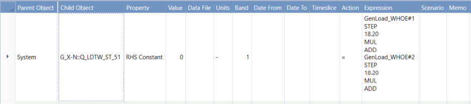
Figure 1: RHS Constant definition for a Constraint
The expression field will accept plain text of any length. It can accept multi-line text, and this is convenient for the readability of the expressions. To type multi-line text use SHIFT-Enter to create new lines while typing. To paste multi-line data, the text must be delimited by quotes. Pasting from a multi-line Excel worksheet cell will preserve the multi-line text.
Expression Syntax
RHS_CONSTANT text expressions are composed of 'tokens', separated by spaces or new lines, and are of two types:
- Operators: listed in the table below, and
- Operands: either numbers or references to variables in the formulation as explained below.
Tokens are organised in the expression according to Reverse Polish notation (RPN). This is a mathematical notation in which operators follow their operands (e.g. a b +), in contrast to Polish notation (PN), in which operators precede their operands (a + b). It does not need any parentheses if each operator has a fixed number of operands.
Example:
Polish notation: a × (b + c) - d
Reverse Polish notation: a b c + × d -
RPN is preferred for processing by computer code. It makes use of a 'stack' (memory) to keep track of operands and processes operators as they are encountered. A stack is a last-in-first-out (LIFO) queue. Items can be pushed onto the stack (in which case the new item becomes the top stack element) or popped off the stack (where the top stack element pops first).
The stack operations for the above example are as follows:
| Token "a" | push "a" on the stack |
| Token "b" | push "b" on the stack - it is now composed to two elements with "b" as the top element |
| Token "c" | push "c" on the stack - it is now composed of three elements with "c" on top |
| Token "+" | pop "c" and "b" from the stack, add them and return the result to the stack - it now has two elements with c+b on top |
| Token "×" | pop c+b and a from the stack, multiply and return the result to the stack - it now has a single element being a×(b+c) |
| Token "d" | push "d" on the stack |
| Token "-" | pop "d" and a×(b+c) from the stack, subtract and return the result to the stack |
The 'result' is read off the top of the stack which is a × (b + c) - d.
Note that when processing RHS_CONSTANT the stack is automatically initialized with one element (0) at the top of the stack.
The supported operators are in Table 1. All the examples shown result in the top stack element ('the result') being 1000.
Table 1: RPN operators| Operator | Name | Operands | Net Stack Effect | Function | Example |
|---|---|---|---|---|---|
| ABS | Absolute Value | 1 | 0 | Pops the top element of the stack takes its absolute value and pushes the result to the top of the stack | "-1000 ABS ADD" |
| ADD | Addition | 2 | -1 | Pops and adds the top two elements of the stack and pushes the result to the top of the stack | "800 200 ADD ADD" |
| DIV | Division | 2 | -1 | Pops and divides the top two elements of the stack and pushes the result to the top of the stack. The denominator is the top stack element, the numerator the second element. | "2000 2 DIV ADD" |
| DUP | Duplicate | 1 | 1 | Increases the stack height by one by duplicating the value of the top stack element | "500 DUP ADD ADD" |
| MAX | Maximum | 2 | -1 | Pops and takes the maximum of the top two stack elements and pushes the result to the top of the stack | "100 900 EXCH ADD ADD" |
| MIN | Minimum | 2 | -1 | Pops and takes the minimum of the top two stack elements and pushes the result to the top of the stack | "1000 500 0 POP EXLEZ EXCH POP ADD" |
| MUL | Multiply | 2 | -1 | Pops and multiplies the top two elements of the stack and pushes the result to the top of the stack | "450 1000 MAX ADD" |
| NEG | Negation | 1 | 0 | Pops the top element of the stack reverses its sign and pushes the result to the top of the stack | "1000 1100 MIN ADD" |
| POP | Pop | 1 | -1 | Pops the top stack element, and if the value is less than or equal to zero sets the flag for the EXLEZ operator to true | "10 100 MUL ADD" |
| RSD | Roll Stack Down | 0 | Moves the top element of the stack to the second to bottom position | "-1000 NEG ADD" | |
| RSU | Roll Stack Up | 0 | Moves the second to bottom element of the stack to the top | "31.62 POW2 ADD" | |
| SUB | Subtract | 2 | -1 | Pops and subtracts the first element from the second and pushes the result to the top of the stack | "10 POW3 ADD" |
| EXCH | Exchange | 2 | 0 | Exchanges the top two stack elements | "2 2000 0 RSD ADD DIV ADD" |
| POW2 | Square | 2 | -1 | Pops and squares the top elements of the stack and pushes the result to the top of the stack. | "2 0 2000 RSU ADD DIV ADD" |
| POW3 | Cube | 2 | -1 | Pops and cubes the top elements of the stack and pushes the result to the top of the stack. | "1000000 SQRT ADD" |
| STEP S | Step function | 1 | 0 | Pops the top element of the stack and pushes 1 if the value is greater than zero otherwise 0 and pushes the result to the top of the stack | "1000 GenLoad_A.1 STEP MUL ADD" |
| SQRT | Square root | 1 | 0 | Pops and takes the square root the top elements of the stack and pushes the result to the top of the stack. | "1500 500 SUB ADD" |
| EXLEZ | Exchange if less than or equal to zero | 2 | 0 | If the POP operator last returned true the EXCH command is performed on the stack | "-1000 ABS ADD" |
Variable References as Operands
Expressions may include references to the solution values of variables in the formulation. For example, you may want to refer to the output of a generator. The reference must exactly match the name of the variable in the formulation and if the name includes spaces you must enclose the references in quotes. Variable names have two parts:
- The prefix: which describes why type of variable it is, and
- The name: which matches the name of the object in the input database.
Most variables can be referenced, and some example references are described in Table 2. The only restriction is that the variable being referenced must have the same indices as the constraint i.e. the constraints are indexed by simulation period and so any referenced variable must also be indexed by simulation period.
Table 2: Example variable references| Reference Type | Prefix | Examples |
|---|---|---|
| Generator Load | GenLoad_ | GenLoad_GenA, "GenLoad_Gen 10" |
| Decision Variable | Var_ | "Var_Region A Load" |
| Line Flow | LinFlow_ | LinFlow_A-B |
Where the value you need is not available as a native variable in the formulation it is convenient to define a Decision Variable to supply the value.
It is important to note that the values of decision variables reference are automatically lagged by one time period i.e. the right-hand side for a constraint in time period t will be computed from solution values of variables from time t-1. However there may be some variables which do not need to be lagged, for example load related variables, where the load values are from a known profile. In this case '{0}' can be appended to the variable, specifying there is no lag applied to this specific variable.
Examples:
Consider a transmission line limit that is set by taking the minimum of two calculated values according to the formulae:
MIN
(1.983 * (Var_Y -0.4992 * (0.0259 * Var_LOAD{0} + 11.69) + 1.32 -
10),
1.725 * (Var_X -0.7426 * (0.0259 * Var_LOAD{0} + 11.69) + 0.07139 -
10)))
Here Var_Y , Var_X and Var_LOAD refer to Decision Variable objects ("Var_" being the prefix for Decision Variable and the remainder being the name of the objects).
The RPN for this is:
"Var_X
-0.7426 0.0259 Var_LOAD{0} MUL 11.69 ADD MUL ADD
0.07139 ADD
-10 ADD
1.725 MUL
Var_Y
-0.4992 0.0259 Var_LOAD{0} MUL 11.69 ADD MUL ADD
1.32 ADD
-10 ADD
1.983 MUL
MIN"
For illustration, assume the decision variable references take these values:
Var_X = 137
Var_LOAD = 1414.09702044226
Var_Y = 141
The stack operations for this expression are as follows:
| (Token: Var_X) | Push 137 | |
| (Token: -0.7426) | Push -0.7426 | |
| (Token: 0.0259) | Push 0.0259 | |
| (Token: Var_LOAD) | Push 1414.09702044226 | |
| (Token: MUL) | Pop 1414.09702044226 | Push 36.6251128294545 |
| (Token: 11.69) | Push 11.69 | |
| (Token: ADD) | Pop 11.69 | Push 48.3151128294545 |
| (Token: MUL) | Pop 48.3151128294545 | Push -35.8788027871529 |
| (Token: ADD) | Pop -35.8788027871529 | Push 101.121197212847 |
| (Token: 0.07139) | Push 0.07139 | |
| (Token: ADD) | Pop 0.07139 | Push 101.192587212847 |
| (Token: -10) | Push -10 | |
| (Token: ADD) | Pop -10 | Push 91.1925872128471 |
| (Token: 1.725) | Push 1.725 | |
| (Token: MUL) | Pop 1.725 | Push 157.307212942161 |
| (Token: Var_Y) | Push 141 | |
| (Token: -0.4992) | Push -0.4992 | |
| (Token: 0.0259) | Push 0.0259 | |
| (Token: Var_LOAD) | Push 1414.09702044226 | |
| (Token: MUL) | Pop 1414.09702044226 | Push 36.6251128294545 |
| (Token: 11.69) | Push 11.69 | |
| (Token: ADD) | Pop 11.69 | Push 48.3151128294545 |
| (Token: MUL) | Pop 48.3151128294545 | Push -24.1189043244637 |
| (Token: ADD) | Pop -24.1189043244637 | Push 116.881095675536 |
| (Token: 1.32) | Push 1.32 | |
| (Token: ADD) | Pop 1.32 | Push 118.201095675536 |
| (Token: -10) | Push -10 | |
| (Token: ADD) | Pop -10 | Push 108.201095675536 |
| (Token: 1.983) | Push 1.983 | |
| (Token: MUL) | Pop 1.983 | Push 214.562772724588 |
| (Token: MIN) | Pop 214.562772724588 | Push 157.307212942161 |
| Result = 157.307212942161 |
Sub expressions
A complex expression that is shared between multiple Constraint right-hand side expressions can be defined using a Decision Variable/Constraint pair and referred to using the "Var_" prefix in your RHS_CONSTANT expressions. To do this, follow these steps:
- Create a Decision Variable with [Objective Function Value] = 0.0 e.g. Decision Variable "INERTIA"
- Create a Constraint of the same name with [RHS] = 0.0 e.g. Constraint "INERTIA"
- Create a membership that puts the Constraint in the Decision Variable's [Definition] collection.
- Define the RHS_CONSTANT on the new Constraint like the following example
Decision Variable "INERTIA" RHS_CONSTANT:
"5.26 GenLoad_OCGT3 STEP MUL ADD
5.26 GenLoad_OCGT2 STEP MUL ADD
5.26 GenLoad_OCGT1 STEP MUL ADD
0.02891 GenLoad_OCGT4 MUL ADD
0.89 GenLoad_OCGT5 STEP MUL ADD
0.89 GenLoad_OCGT6 STEP MUL ADD
7.89 GenLoad_OCGT7 STEP MUL ADD
14.61 GenLoad_OCGT8 STEP MUL ADD
31.4 GenLoad_CCGT STEP MUL ADD
GenLoad_CCGT -237 ADD STEP 16.29 MUL ADD
0.0362 GenLoad_OCGT9 MUL ADD
2.09 GenLoad_OCGT10 STEP MUL ADD
0.89 GenLoad_OCGT11 STEP MUL ADD
0.89 GenLoad_OCGT12 STEP MUL ADD
0.89 GenLoad_OCGT13 STEP MUL ADD
0.89 GenLoad_OCGT14 STEP MUL ADD
10.065 GenLoad_OCGT15 STEP MUL ADD
0.02 GenLoad_OCGT16 MUL ADD
7.95 GenLoad_STA1 STEP MUL ADD
7.95 GenLoad_STA2 STEP MUL ADD
7.95 GenLoad_STA3 STEP MUL ADD
7.95 GenLoad_STA4 STEP MUL ADD
9 GenLoad_STB1 STEP MUL ADD
9 GenLoad_STB2 STEP MUL ADD
9 GenLoad_STB3 STEP MUL ADD
9 GenLoad_STB4 STEP MUL ADD
0.52 GenLoad_OCGT18 STEP MUL ADD
0.014 GenLoad_OCGT17 MUL ADD"
You can now use this expression in other RHS_CONSTANT expressions by referring to its name e.g. "Var_ INERTIA" as in the following example for Constraint "ROCOF":
"1
3
100 Var_INERTIA MUL ADD
0.04 MUL MUL ADD
1
3
100 Var_INERTIA MUL ADD
0.04 MUL
24 ADD MUL
1
1 STEP MUL
POP
EXLEZ
EXCH POP"
Flow of Execution
Constraints that define RHS_CONSTANT are enforced iteratively along with other similar constraints (such as transmission constraints) during the simulation process. An iterative approach is used, first solving with no constraints in the formulation, then checking for violations by computing the current value of the right-hand side (based on the result of the expression plus any input right-hand side part) and adding constraints if violations are detected and repeating until all constraints are enforced and no right-hand side values require further updating.
Convergence
Right-hand side constants based on complex expressions can result in a different convergence process than regular constraints i.e. those with fixed right-hand side values. With regular constraints, the addition of new limits increases the objective function value every iteration and convergence is achieved as soon as either:
- no more constraints are violated, or
- the problem is infeasible.
In particular, it is constraint right-hand side expressions that include integer switches (such as the STEP, MIN, MAX operators) can lead to situations where the simulation cycles between solutions or fails to fully converge after many iterations.
The simulation program detects when cycling is occurring according to the following rules:
- If an iteration returns an objective value equal to any previous iteration, the iterations are stopped (as in Figure 3).
- If the absolute value of the change in objective function between iterations begins to increase (rather than decreasing as expected in a linear system) the iterations can continue until the next time the objective function ticks up and which point the iterations are stopped (Figure 4).
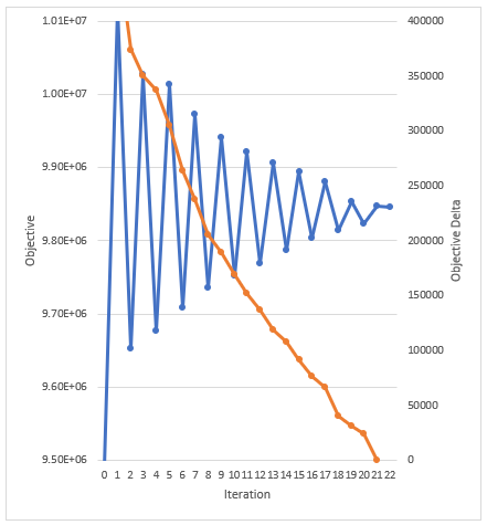
Figure 3: Convergence
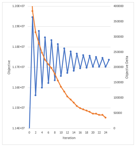
Figure 4: Nonconvergence due to cycling
Progress Messages and Reporting
There are two Diagnostic switches that apply to constraint iterations as highlighted in Figure 5. The option [Monitored Iterations Summary] prints a one-line summary at the conclusion of constraint convergence, whereas [Monitored Iterations] prints messages for each iteration as in the following example:
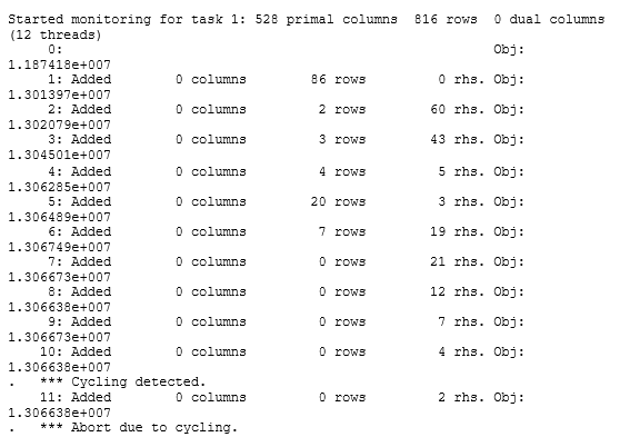
Figure 5
Here "columns" is the number of new variables added, "rows" the number of new constraints and "rhs" is the number of previously-added constraint right-hand side values updated in the iteration. "Obj" is the objective function value.
11. Decision Variables
The Decision Variable class creates user-defined variables in the mathematical programming formulation. These variables can be used for a wide variety of modelling purposes including:
- Modeling commodities with a demand such as desalination as a product of electric power and heat.
- Modeling the storage electricity or any other commodity.
- Calculating values that are functions of intrinsic decision variables and passing these to the solution.
- Cancelling out default objective function coefficients by defining a decision variable to be equal to an intrinsic variable with the opposite objective function term.
- Enforcing integer restrictions on decision variables that are intrinsically linear.
- Modeling piecewise or general non-convex or discontinuous functions.
To key property for Decision Variable is Objective Function
Coefficient although you may simply set this to zero if desired. Other
important properties are Lower Bound and Upper Bound and Type (linear
or integer).
Once the variable is defined you may use it in Constraint objects or
'inject' the variable into the built-in formulation.