Interface Class
| Description: | Transmission interface |
See also Interface Property Reference for a detailed list of properties for this class of object.
Interfaces
An Interface is a collection of lines (AC and/or DC) in the transmission network that together deliver power from one area to another. There are limits on the combined flow across the interface in either direction.
- Each AC or DC line has a notional direction for positive flows.
- The collection of lines in the interface can involve lines that notionally flow in the same or opposite way to the interface.
- Interface flow is usually described as being the net flow (i.e. sum of all flows [positive or negative]) across the lines in the interface, although PLEXOS provides functionality to define the interface flow in any way.
To define an interface, you first create a new Interface object using the new Interface object using the New Interface Wizard available from the right mouse button pop-up menu for the Interfaces collection. Add all AC and DC lines (regardless of their notional flow direction) during this step.
Example
| Interface | Property | Value | Units |
| ABC | Max Flow | 1000 | MW |
| ABC | Min Flow | -900 | MW |
| Interface | Line | Property | Value | Units |
| ABC | L1 | Flow Coefficient | 1 | MW/MW |
| ABC | L2 | Flow Coefficient | -1 | MW/MW |
| ABC | L1 | Flow Coefficient | 1 | MW/MW |
The properties Min Flow and Max Flow must be defined for PLEXOS to include the interface in the set of constraints for the Model. For example, you can use the Scenario field here to tag these properties so that the Interface can be considered only when you include the appropriate Scenario(s) in your Model. The Interface Lines property is used to set the coefficient in the constraint equation:
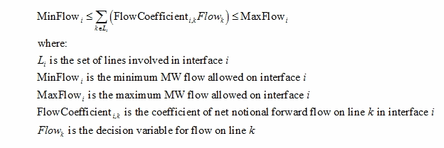
Line flow is defined as positive for flows from the Node From to the Node To and negative for reverse flows. Thus the flow coefficients in the interface need to be set correctly taking this notional line direction into account.
Any coefficient can be used (not just 1 or -1). It is possible to set the coefficient on flows 'forward' and 'backward' on line flows differently using the Interface Lines properties, as shown in the following equation:
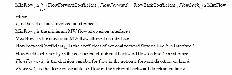
The decision variables for line flow are non-negative, e.g. when the line is flowing forward. The variable for the line flow backward receives a negative value. In other words, when we change this line to have a Flow Back Coefficient, in reference to the Interface, we get a negative value in the Interface.
The minimum and maximum flow limits on the interface may vary in time just as any input property in PLEXOS. However, the Interface class itself does not directly support dynamic limits, i.e., limits that are a function of demand and/or generator output. These limits are instead handled with the Constraint class, as discussed in the following section.
Note that you can globally toggle on/off consideration of interface flows limits using the Transmission Interface Constraint Enabled property.
Dynamic Interface Limits
Use of Constraint objects to model transmission interfaces allows modeling of dynamic min and max flows.
The simulator models transmission lines with two sets of variables, one for flows in the notional forward direction, and one for flows in the notional backward direction. These variables can be included in generic constraints and this is the mechanism used to model interfaces using constraints. The line objects included in the interfaces are added to a constraint object's Lines collection, and the appropriate coefficients are set on those lines' flows to define the interface constraint. Because the flow directions are separate variables in the formulation, there must be one constraint for each direction of flow on the interface i.e. a forward interface constraint, and a backward interface constraint.
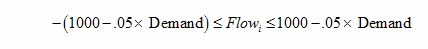
Consider an example in which three lines form an interface. L1, and L3 have the same notional flow direction as the interface, but L2 has the opposite notional flow direction. Assume the interface is called "I" and that its limit is a function of regional demand as in the following equation:
This system can be set up thus:
- Create a Constraint object called "I+" to represent flow forward and add the Lines L1, L2, and L3 to the Constraint's Lines collection.
- Create a Constraint object called "I-" to represent flow forward and add the Lines L1, L2, and L3 to the Constraint's Lines collection.
- For I+ set the properties on the Constraint's Lines shown in Table 3.
- For I- set the properties on the Constraint's Lines shown in Table 4.
- Set the properties for the Constraints' themselves shown in Table 5. The Sense property = -1 indicates that this is a less-than-or-equal to constraint. The RHS properties are the constant part of the transmission limit in each direction.
Note how the coefficients on the Lines are set recognizing the notional direction of those lines relative to the direction of the interface.
| Class | Name |
| Constraint | I+ |
| Constraint | I- |
Table 1: Interface Constraint Objects
| Collection | Parent Name | Child Name |
| Line.Constraints | I+ | L1 |
| Line.Constraints | I+ | L2 |
| Line.Constraints | I+ | L3 |
| Line.Constraints | I- | L1 |
| Line.Constraints | I- | L2 |
| Line.Constraints | I- | L3 |
| Region.Constraints | I+ | R |
| Region.Constraints | I- | R |
Table 2: Constraint Memberships
| Constraint | Line | Property | Value | Units |
| I+ | L1 | Flow Coefficient | 1 | - |
| I+ | L2 | Flow Back Coefficient | 1 | - |
| I+ | L3 | Flow Coefficient | 1 | - |
| I- | L1 | Flow Back Coefficient | 1 | - |
| I- | L2 | Flow Coefficient | 1 | - |
| I- | L3 | Flow Back Coefficient | 1 | - |
Table 3: Constraint Lines Properties
| Constraint | Line | Property | Value | Units |
| I+ | R | Demand Coefficient | .05 | - |
| I- | R | Demand Coefficient | .05 | - |
Table 4: Constraint Regions Properties
| Constraint | Property | Value | Units |
| I+ | Sense | -1 | - |
| I+ | RHS | 1000 | - |
| I- | Sense | -1 | - |
| I- | RHS | 1000 | - |
Table 5: Constraint Properties
Example
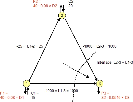
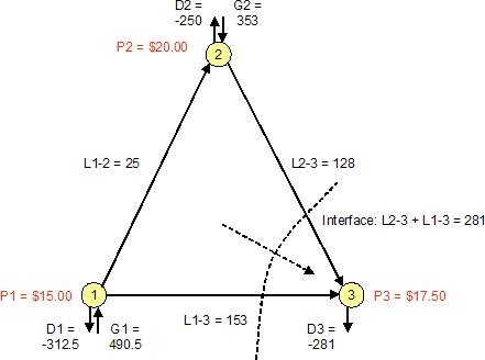
The following is a simple three-node model. There is generation at nodes 1 and 2, and demand at all nodes. The lines in this AC network have equal susceptance, and flows must obey Kirchhoff's Laws. The demand at each node is represented by demand functions.
The lines leading into node 3 have individual limits, but for the purposes of this example we shall assume that the combined flows into and out of node 3 form an interface with an upper limit of 250MW and a lower limit of -100MW. The second figure shows the optimal flows ignoring the interface constraint but obeying the individual line limits. The total flow across the interface is 281MW (153 + 128).
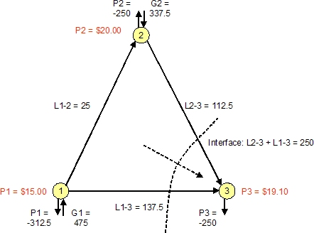
In the last figure, the interface constraint is enforced, and the flows across L2-3 and L1-3 fall, while the price at node 3 rises to 19.10 from 17.50.
Ramp
The rate-of-change of Flow, or Ramp, can be controlled by these properties:
- Max Ramp Down and Max Ramp Up : which define hard limits on the ramp; and/or
- Ramp Penalty which penalizes ramp.