Nodal Transmission Diagnostics
The Transmission Diagnostic table provides the capability to selectively create diagnostic output related to the loading of transmission elements in nodal studies. There are several categories of output available: NodalDiagShiftFactor, NodalDiagLODF, NodalDiagLoadSource, NodalDiagContinencyFlow.
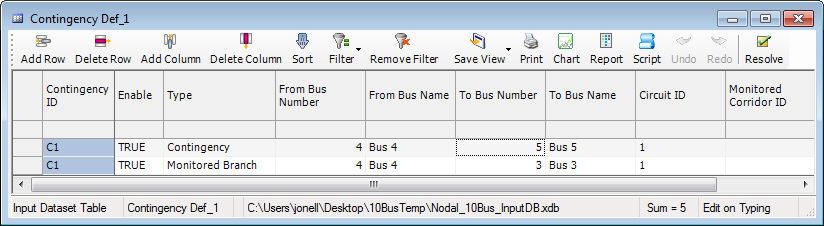
Contact Support to get an archived project of the following example. With that project you can follow this example relating to contingencies that should help you understand the use of the Transmission Diagnostic table and the three output tables. First, look at the contingency table in the database:
The Transmission Diagnostic table as follows:
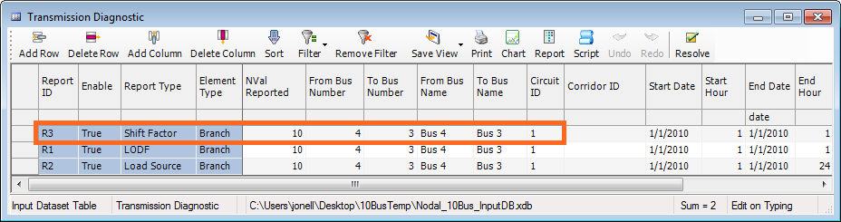
The first line tells the model to report the most important shift factors relating to branch 4_3_1.
The output table is NodalDiagShiftFactor and looks like this after running:
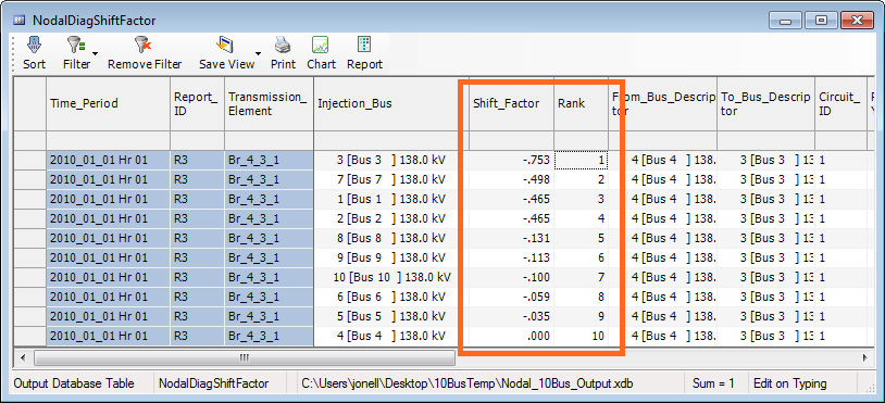
The shift factors are shown, in order of most influential to least influential buses on the line. Since this data does not change unless our topology changes, you only need to report this for multiple hours if the topology changes.
The second line of the Transmission Diagnostic table says to report the LODF(s) for the branch from bus 4 to bus 3 in relation to all contingencies. In this case there is only one contingency, and so we will expect to see just one unique LODF in the NodalDiagLODF output table. This is what appears in the output:
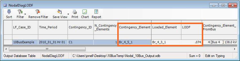
This shows that 7.4% of the flow on branch 4_5_1 will be transferred to 4_3_1 in the event of the contingency.
The third line of the Transmission Diagnostic table as seen above will report the information from the previous two tables plus more. It reports information about the buses which cause the most induced flow on the branch (either direction). It will also report information about contingencies. This information will change on an hourly basis because it is based on the net_injections at the buses. Here is what the NodalDiagLoadSource output looks like:
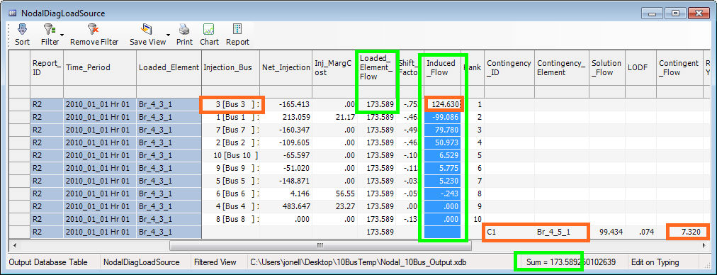
This shows, in order, the most significant contributors to flow on the branch 4_3_1. See that the highest contributor to flow was Bus 3 (at the top), with induced flow of:
[Bus 3 Net Injection] * [Shift Factor] = (-165.413) * (-.753) = 124.63 MW
In this case since there are only ten buses in the system, all contributors to flow are listed here, and the sum of the Induced_Flow column (highlighted in green) is equal to the Loaded_Element_Flow column.
The last line in this table shows that in the event of the contingency C1 (i.e. loss of branch 4_5_1) then 7.32 MW of additional flow would come on branch 4_3_1
[Flow on branch 4_5_1] * [LODF] = 99.434 * .074 = 7.32 MW
So from this output table you can get all the information you need about what buses are contributing to flow on a line and what the effect a contingent element would have on line flow.
![]() Nodal Transmission Diagnostics
Nodal Transmission Diagnostics