Marginal Losses Method

This specifies whether marginal losses will be calculated in a Nodal study. Use the drop down to select None, PenaltyFactors, or Dynamic Losses.

NOTE: The option to Use Distributed Slack Bus, found in the Solution Settings folder of Simulation Options, must be selected for use when running with Penalty Factors for marginal losses.

Aurora offers two options for modeling losses in the nodal model. One is a static penalty factor approach and the other is a dynamic approach which also uses penalty factors. The static approach has the main advantage of being faster while the dynamic approach produces a higher quality of results and is ideal for longer simulations.

First, at the core of both approaches is the concept of penalty factors and loss sensitivities. The loss sensitivity for bus i is the change in system losses with respect to a change in net injection at the bus.

Specifically, look to the following formula:

where LSi is the loss sensitivity, L represents system losses, and NI represents net injection.

The loss sensitivity will be positive for buses which increase system losses by injecting power into the grid and negative for buses which decrease system losses by injecting power into the grid.

The penalty factor at bus i is related to the loss sensitivity as follows:

So, positive loss sensitivity implies a penalty factor that is greater than 1 and negative loss sensitivity implies a penalty factor that is less than 1. Penalty factors should always be positive numbers and ideally should not be significantly greater than 1.

These numbers are used in slightly different ways per method used in Aurora. An important use of these numbers that both methods share in common is in the calculation of the loss component of LMP.

So, a positive loss sensitivity or penalty factor of greater than 1 implies a negative marginal cost of losses given that typically the marginal cost of energy is positive. A negative loss sensitivity or penalty factor of less than 1 implies a positive marginal cost of losses.

In other words, the marginal cost of losses will be negative if you are electrically distant from load and it will be positive if you are electrically close to load.

Static Approach - "Penalty Factors"

The penalty factor approach to marginal losses consists of a preliminary hour simulation to calculate penalty factors at every bus in the system. Once they have been calculated the model begins its simulation and applies the penalty factors to generator costs. Click here for more information.

The calculation of penalty factors consists of the following steps:

A nodal solution without contingencies (n-0) solution is determined for the hour corresponding to the median load for the first calendar year of the study.
System losses are calculated as a function of line resistance and MW flows and distributed to demand buses (see Note below for more detail).
Another nodal solution for the same hour is attempted with losses added to the system.
Using the solution from step 3, loadflows are calculated for every bus in the system to determine the change in system losses arising from increasing the injection of power at each bus individually by 1 MW. This gives the quantity d(SystemLosses)/d(InjectionBusi).
Penalty Factors for every bus are calculated as 1/(1-d) where d is the d(SystemLosses)/d(InjectionBusi) quantity calculated in step 4.

Once penalty factors are calculated the model begins at the study start date. The following changes are applied in order to arrive at the marginal cost component of LMP:

System losses are estimated by aggregate area as a percentage of hourly demand derived from the initial penalty factor calculation step. The losses are added to the system as extra demand.
Penalty factors are applied to generator costs in the following manner: Cost Gen i = Initial Cost Gen i * Penalty Factor Gen i. Note that penalty factors typically are around 1. A value higher than 1 indicates that it costs more to operate a generator due to the effect of losses. A value less than 1 indicates that it costs less to operate a generator due to the effect of losses.

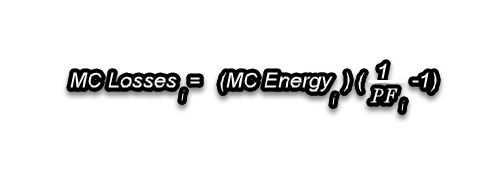
Finally, the marginal loss component of LMP is calculated as:

LMP marginal loss = LMP energy * (1/PFi - 1)

where PFi is the penalty factor for bus i

NOTE: The method with which losses are distributed in the penalty factor calculation process finds the path with smallest amount of resistance to a demand bus and places losses weighted by flow magnitude. The net result is that losses get placed as extra demand at buses connected to branches as a function of flow magnitude on the branch. The loss factor is the aggregate area level loss divided by the aggregate area level demand.

Dynamic Approach - "Dynamic Losses"

The dynamic losses approach is basically the same as the up-front penalty factor loop used in the above method except that it is performed every hour. In doing this, Aurora recognizes contingencies when they are being used and is able to use the zonal commitment logic as well as any nodal informed commitment decisions. Loss sensitivities are still used here in order to calculate the loss component of LMP and penalty factors are applied to generator costs (lagged by one hour due to the timing of calculations). Click here for more information.

The basic process is, for N-0 :

Do a lossless solution. This includes determining which branch or corridor constraints need to be included.
Calculate losses and distribute* them as additional bus demand. *The loss distribution method places branch losses 50/50 on its end buses. This will turn every bus in the system into a demand bus and might require a recalculation of shift factors and LODF’s. This approach differs from the Penalty Factors method.
Do a solution including losses. This step also includes finding new branch or corridor violations which might have been caused by the addition of losses.
Compare system losses as a percentage of demand to that of the previous iteration and branch losses to those from the previous run. If the system losses delta is smaller than the user input tolerance and there are no branches with loss deltas exceeding the user input tolerance, then the process is complete. If not return to step 2. Alternatively, if the tolerance values are never met the max number of iterations is used.
When finished, calculate loss sensitivities.

NOTE: If monitoring radial lines, a check is made so that losses will not be placed at the end of a radial line that cause the total demand at the end to exceed the line limit.

The process for SCOPF is similar :

Do the process for N-0 as described above.
Do a SCOPF loop with losses from the N-0 solution in step 1.
Calculate losses and distribute them as additional bus demand.
Do another SCOPF loop.
Compare system losses as a percentage of demand to that of the previous iteration and branch losses to those from the previous run. If the system losses delta is smaller than the user input tolerance and there are no branches with loss deltas exceeding the user input tolerance, then the process is complete. If not return to step 4. Alternatively, if the tolerance values are never met the max number of iterations is used.
Compute loss sensitivities when finished.

NOTE: Lines that are not monitored will not contribute losses to the system in order to avoid a potentially significant contribution of losses to the system that is not reasonable. They will also not contribute to loss sensitivities.

NOTE: Using different slack buses can produce differences in results when using dynamic losses even when the shift factor tolerance is set to 0. This is due to an internal tolerance for system loss level convergence as opposed to requiring that convergence is achieved with a 0 tolerance at every branch in the system.

Simulation Options

Nodal

Marginal Losses Method