LOLP Statistics
Contents
- Introduction
- Reliability Indices
- Local versus Multi-area LOLP
- LOLP Versus Monte Carlo
- Setup
- Intermittent Generation
- Example
1. Introduction
The Loss of Load Probability (LOLP) and related statistics are calculated in the PASA phase of the simulator using convolution via the Capacity Outage Probability Table (COPT) method. The expected energy not served (EDNS) is also computed, indicating the expected severity of outages.
This article discusses the application of the LOLP to reliability studies and comparison to Monte Carlo simulation.
2. Reliability Indices
Four reliability indices are computed:
LOLP
The probability that demand will exceed the capacity of the system in a given period.
LOLE
The loss of load expectation index is the number of days of outage and is calculated directly from the LOLP:
LOLE = LOLP * t / 24
where:
t is the number of hours in the PASA time block.
24 converts hours to days
EDNS
This is the expected megawatt demand not served in the PASA period i.e. the expected outage severity. The EDNS is determined by taking the total area where the demand is greater than the available capacity Region Available Capacity.
EENS
This is calculated directly from the EDNS:
EENS = EDNS x t
where:
t is the number of hours in each PASA time block.
3. Local Versus Multi-area LOLP
Two versions of LOLP calculation algorithm are available:
The key points of difference between the local and multi-area reliability algorithms are the treatment of transmission and the output reliability metrics.
The local LOLP algorithm reads the transmission reserve capacity 'flows' from the PASA solution. The net import implied by these reserve flows is subtracted from the local load and the LOLP is computed on this net load.
The multi-area LOLP also considers the flow limits, but solves interconnected regions together, thus considering the probability of failure of units providing support to neighbouring regions. These flows are bounded by the input Line Max Flow, Min Flow and/or Min Rating, Max Rating. It calculates only the LOLP and the derived LOLE statistics. It does not calculate the outage magnitude statistics EDNS and EENS.
Figure 1 shows how EENS is correlated with LOLP. The relationship is approximately polynomial, which seems intuitive i.e. higher LOLP implies increasingly severe outage magnitude.
If outage severity statistics are important in your model it is desirable to use the local LOLP algorithm. The question remains, however, of how to account for the reliability of generators providing capacity support via transmission?
A reasonable solution to this is to use conservative transmission limits derived from Monte Carlo simulation with a full transmission model with constraints. The Line Import Limit and Export Limit reported out of that run can be input as limits to the LOLP Run. The most conservative approach would be to take the minimum limits in each period across the thousands of Monte Carlo simulations.
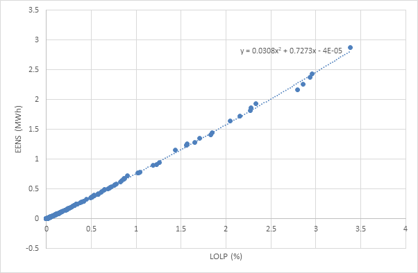 Figure 1: EENS relationship to LOLP
4. LOLP Versus Monte Carlo
The LOLP algorithm and Monte Carlo both seek to estimate the probability and severity of outage events. LOLP is 100% accurate with respect to the COPT, but it does not account for all constraints on generation and transmission. Monte Carlo accounts for all types of constraints but takes the combined results of many outage patterns (samples/iterations) to converge.
Figure 2 compares the EENS figure from the LOLP algorithm against the average Unserved Energy from 2000 Monte Carlo simulations for the same run as in Figure 1. Although the average values are similar, the Monte Carlo exhibits more severe events. Monte Carlo is the preferred method, providing an estimate that accounts for all system constraints whereas EENS is a good "quick and dirty" estimate.
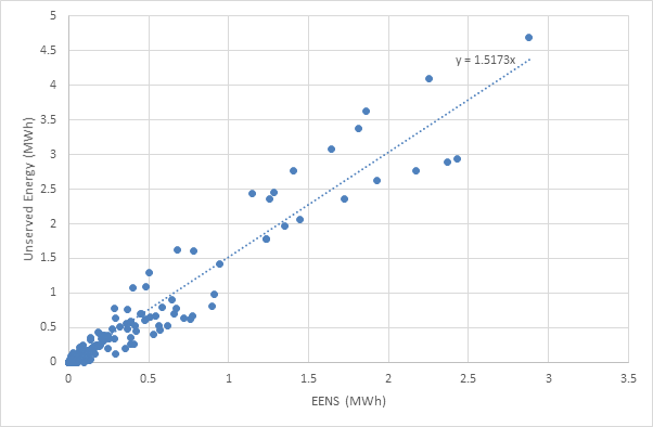 Figure 2: EENS versus Monte Carlo Unserved Energy
5. Setup
The Horizon should be set up to run for the required duration and interval length. An example is shown in Figure 3 for a one-year horizon at hourly resolution.
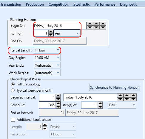 Figure 3: Example Horizon settings
The PASA simulation phase calculates the loss of load statistics. The phase is set up with interval resolution and options toggled on so that reliability statistics are computed as shown in Figure 4.
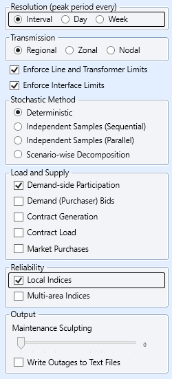 Figure 4: PASA Settings for LOLP Run
Required non-default settings:
- Step Type = 0 ("Interval"): This will cause PASA to calculate at the resolution of Horizon [Periods per Day].
- Compute Reliability Indices = "Yes": Invokes calculation of LOLP and other statistics assuming full import on interconnectors with 100% reliability.
These PASA reliability settings work with the corresponding reliability indices on the Region/Zone report selections shown in Figure 5.
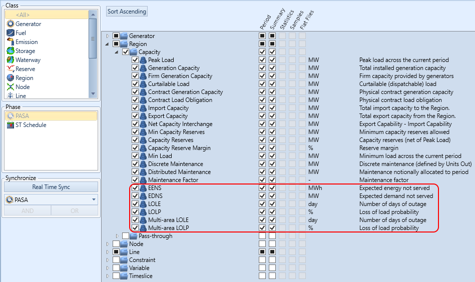 Figure 5: Region Report settings
LOLP uses a similar set of input data to Monte Carlo, which is described in the section on basic and optional inputs. It supports full and partial outage states.
6. Intermittent Generation
Whereas thermal generators have well-defined outage states ('on', 'off', or 'partial') with defined probabilities, renewable generation can be limited to practically any megawatt output in its feasible range. This can be dealt with by creating outage "buckets" for the renewables, with associated probabilities and then treating each bucket as a pseudo-generator in the LOLP calculation.
Consider the following example. Historical wind speed data implies that, on the dispatch interval of peak electrical demand, wind production could vary between zero and two megawatts with distribution as shown in the blue bars in Figure 6.
For illustration only, the orange bars in Figure 6 represent a normal distribution fit to the data (μ=0.75, σ=0.44). This fit can be translated into the Table 1 Generator Outage Rating and Forced Outage pairs.
NOTE: An alternative to Outage Rating which is a megawatt figure, is Outage Factor which is a 'simple' percentage outage and can be more convenient to use, especially with template objects.
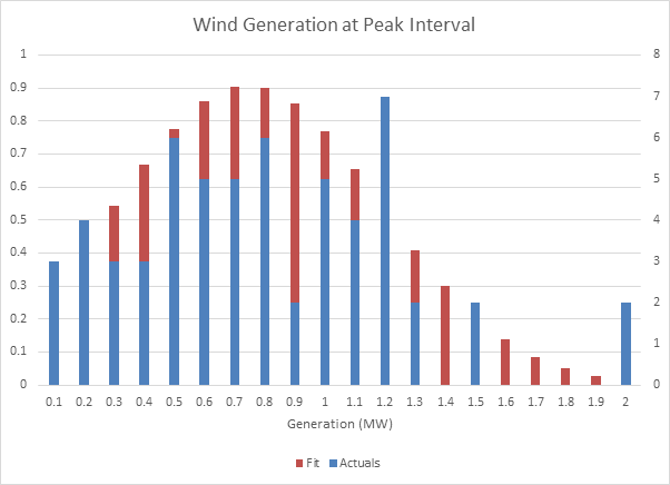 Figure 6: Wind Generation at Peak Interval
Table 1: Input data for intermittent generation
| Property | Value | Unit | Band |
|---|---|---|---|
| Forced Outage Rate | 4 | % | 1 |
| Forced Outage Rate | 3 | % | 2 |
| Forced Outage Rate | 3 | % | 3 |
| Forced Outage Rate | 5.1 | % | 4 |
| Force Outage Rate | 6.1 | % | 5 |
| Forced Outage Rate | 7.1 | % | 6 |
| Forced Outage Rate | 9.1 | % | 9 |
| Forced Outage Rate | 8.1 | % | 8 |
| Forced Outage Rate | 9.1 | % | 9 |
| Forced Outage Rate | 9.1 | % | 10 |
| Forced Outage Rate | 8.1 | % | 11 |
| Forced Outage Rate | 7.1 | % | 12 |
| Forced Outage Rate | 6.1 | % | 13 |
| Forced Outage Rate | 5.1 | % | 14 |
| Forced Outage Rate | 4 | % | 15 |
| Forced Outage Rate | 2 | % | 16 |
| Forced Outage Rate | 2 | % | 17 |
| Forced Outage Rate | 1 | % | 18 |
| Forced Outage Rate | 1 | % | 19 |
| Forced Outage Rate | 0 | % | 20 |
| Outage Rating | 0 | MW | 1 |
| Outage Rating | 0.1 | MW | 2 |
| Outage Rating | 0.2 | MW | 3 |
| Outage Rating | 0.3 | MW | 4 |
| Outage Rating | 0.4 | MW | 5 |
| Outage Rating | 0.5 | MW | 6 |
| Outage Rating | 0.6 | MW | 7 |
| Outage Rating | 0.7 | MW | 8 |
| Outage Rating | 0.8 | MW | 9 |
| Outage Rating | 0.9 | MW | 10 |
| Outage Rating | 1 | MW | 11 |
| Outage Rating | 1.1 | MW | 12 |
| Outage Rating | 1.2 | MW | 13 |
| Outage Rating | 1.3 | MW | 14 |
| Outage Rating | 1.4 | MW | 15 |
| Outage Rating | 1.5 | MW | 16 |
| Outage Rating | 1.6 | MW | 17 |
| Outage Rating | 1.7 | MW | 18 |
| Outage Rating | 1.8 | MW | 19 |
| Outage Rating | 1.9 | MW | 20 |
NOTE: The raw probabilities and outage ratings could be entered in the bands, it is not necessary to fit a distribution to the data, this is shown as for illustration only as it may be a convenient way to produce the input from raw wind speed data.
7. Example
Results of LOLP calculation by hour are shown in Figure 7.
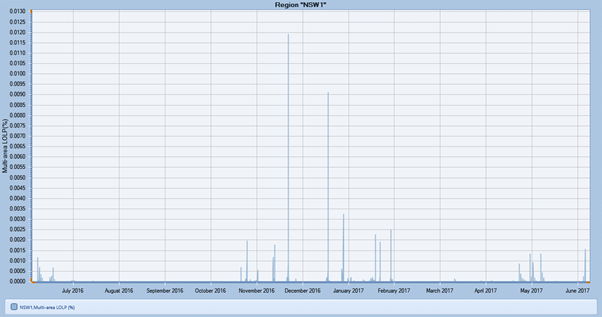 Figure 7: Example LOLP results
See also: Monte Carlo Simulation