PASA Class
| Description: | PASA simulation phase |
See also PASA Property Reference for a detailed list of properties for this class of object.
Introduction
PASA is an acronym for Projected Assessment of System Adequacy. The PASA is closely related to the similarly named models used in the Australian NEM for reporting short and medium term capacity adequacy but its algorithm is applicable to all markets/systems.
The functions of the PASA simulation phase are:
- to create maintenance events for the subsequent simulation phases MT Schedule and ST Schedule
- to compute reliability statistics such as LOLP for the system
For two reasons, PASA is not a value-based reliability (VBR) maintenance optimization:
- The objective function of PASA only deals with capacity reserve margin and not production cost.
- The key output of PASA is the Region Maintenance Factor which is used to shape randomly generated maintenance events into periods of time with high reserve margin. Thus every Monte Carlo sample will have a slightly different maintenance pattern.
Value-based reliability style of maintenance optimization is available through the Maintenance class of objects and integrates directly in MT Schedule and/or ST Schedule.
The input properties that drive the maintenance function are described in the article Planned and Random Outages.
NOTE: PASA computes reliability indices such as LOLP only when the attributes Compute Reliability Indices and/or Compute Multi-area Reliability Indices are enabled.
Algorithm
The PASA uses results of an optimization that focuses on the balance of supply and demand in the medium term. It can be run alone, or as a phase in a more detailed simulation. It produces output such as the projected Capacity Reserves (capacity in excess of Peak Load) and LOLP on a area-by-area basis. You can configure PASA to run at various transmission detail levels with the Transmission Detail setting. The default is Region but Zone and Node are also available. In the following we refer to "area" as a generic term for the transmission detail type, and linked properties are for the Region class by apply equally to Zone and Node.
In multi-area models PASA also calculates the optimal amount of reserve that should be shared between areas using the transmission network. The PASA does this by formulating the problem of equalizing area capacity reserves as a quadratic programming (QP) problem. The quadratic part is essentially a least-squares calculation where the relative deviation of capacity reserves from a constant level is the metric being minimized.
NOTE: If the Performance SOLVER does not support quadratic programming the optimization task is reformulated as a piecewise linear programming problem.
PASA always runs in annual steps across the whole planning horizon: as defined by properties of the horizon being run. The default resolution is one period per day but this can be set to week or interval if required using the Step Type setting. PASA divides the planning horizon into equal sized steps, each being one year. For example, if daily resolution is used over a two-year horizon PASA will solve in two steps each of 366 notional days (with non-leap years containing a notional empty 29th February).
Formulation
The objective of the PASA optimization is to equalize Capacity Reserves across all peak periods i.e. daily, weekly or monthly peak interval.
Area Capacity Reserves is the spare generation capacity over and above Peak Load. The Capacity Reserve Margin is the same quantum expressed as a percentage of the Peak Load.
Generator objects are 'dispatched' for capacity reserves up to their maximum or to their Firm Capacity less their expected Forced Outage. Inter-area lines are used to arbitrage capacity reserves such that reserve levels are equalized across areas taking into account the relative size of units in each area i.e. an area with large units might receive more reserve than one with smaller units. Intra-area lines are ignored. Only if Transmission Detail = "Nodal" are all connections considered but in all cases a simple transportation model of flows is used.
Controlling Parameters
As alluded to above, generators such as wind, solar, etc, whose firm capacity is less than their simple Installed Capacity (based on Max Capacity can have their Firm Capacity defined directly, where this value is per generating unit.
The Line property Firm Capacity can be set to hardwire a particular level of reserve sharing between areas. Variable generator and line ratings are considered but energy constraints are excluded, because the PASA is concerned with instantaneous capability not energy.
Generic transmission Constraint objects are excluded by default but can be included by setting the Include in PASA property.
The property Min Capacity Reserves can be used to set the priority of area for capacity reserves i.e. regions with a high minimum capacity reserve will tend to receive more reserve. Alternatively use the Min Capacity Reserve Margin.
The PASA accounts for planned generator outages. It also calculates how much generator maintenance needs to be scheduled from the Maintenance Rate input and allocates this across each step of the simulation, again with the objective of equalizing region/zone reserves. To ensure maintenance stays within capacity during the PASA phase, it is essential to explicitly define the Max Total Maintenance Percent or Min Total Maintenance Percent property.
You can control the amount of maintenance assigned to a company in any one period with the properties Max Maintenance and Min Maintenance.
The distribution of maintenance outages is optimized by PASA and the idealised shape is reported as the Maintenance Factor output. This property though can be input directly and the distribution of maintenance outages controlled.
PASA Output
When used in combination with MT Schedule and/or ST Schedule, the primary purpose of the PASA is to determine, where and when maintenance outages should occur, taking into account peak load, available capacity, transmission capacity, and any other constraints including transmission constraints.
But PASA is a useful planning model in itself and produces a wide range of output. At execution time PLEXOS creates new objects in the solution database: PA Region/PA Zone, PA Generator, etc. The PASA solution is reported on these objects.
In addition, PASA produces a short report for each area at each simulation step. This report can be used to determine the size and timing of capacity shortfalls i.e. it indicates when new capacity is required. An example report is:
Region NSW1:
Minimum Reserve on 13-Jul-2003
Maximum Demand             12490.00 MW
Demand Curtailed           0.00 MW
Generator Reserve          12202.00 MW
Net Reserve Interchange    -2680.09 MW
Discrete Maintenance       0.00 MW
Distributed Maintenance    544.09 MW
Reserve Trigger Level      660.00 MW
Reserve                    1848.00 MW
Reserve Margin             14.80%
In this case PASA reports that the maximum demand for the region occurs on July 13, 2003. The remainder of the report breaks out all the components of reserve.
When reserves fall below the trigger level the following report is produced:
Region NSW1:
Minimum Reserve on 12-Jan-2009
Maximum Demand             14570.00 MW
Demand Curtailed           0.00 MW
Generator Reserve          12195.00 MW
Net Reserve Interchange    -2317.00 MW
Discrete Maintenance       0.00 MW
Distributed Maintenance    0.00 MW
Reserve Trigger Level      700.00 MW
Reserve                    -58.00 MW
Reserve Margin             -0.40%
*** Capacity Required      758.00 MW
Here the reserve has fallen below the minimum capacity reserves and PASA reports that capacity is required to make up the shortfall. Note that PASA notionally adds this capacity into the area for the next PASA step so that reserve sharing is not unduly biased by area with reserve shortfalls. Thus shortages reported incremental not cumulative. This notional new capacity is not carried through to MT Schedule or ST Schedule.
Maintenance Scheduling
The key output of PASA is the Region Maintenance Factor. This value is simply the normalised inverse of the Region Capacity Reserves. An example is shown in Figure 1.
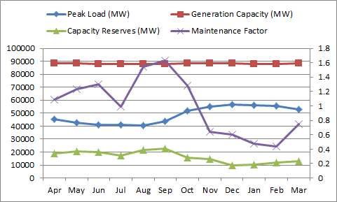 Figure 1: Example Maintenance Factor and Capacity Reserves
The higher the maintenance factor the better the period is for a maintenance event. A maintenance factor value of one means that a time period is 'neutral', whereas values less than one mean that maintenance is discouraged, and when maintenance factor is zero no maintenance events can occur in the period.
In Monte Carlo simulation (where the sample size is set by Stochastic Risk Sample Count) the PASA generates a set of maintenance outage events for each unreliable object (Generator, Line, Gas Pipeline). The frequency and duration of the outages is controlled by properties of those objects as described in the article Planned and Random Outages.
The exact algorithm for placing maintenance outages in time is controlled by the Monte Carlo Method. The methods available share the same basic concept which begins by calculating the mean time between failures (MTBF):
Mean Time Between Failures = (1 - Maintenance Rate) * Mean Time to Repair / Maintenance Rateand then following this algorithm:
- Draw a random number (r) to find the time between failures for the current and last events e.g. if MTBF = 200 hours and r = 0.6 then the time between the last and next failure is 120 hours.
- Modify this 'raw' time to failure by looking up the value against the Maintenance Factor. This is simply a process of adding up the maintenance factor values until the start hour required is reached. For example if the maintenance factor equals 2 for the first 100 hours, then adding up these values will find we reach 120 hours in the 60th actual hour, thus the time to failure would be 'compressed' in this period causing events to accumulate in that time, whereas if the maintenance factor were 0.5 for the first few hundred hours, our time to failure of 120 would be spaced out to the 240th hour.
- Move forward in time to the end of the current failure and return to Step 1 until the horizon has been populated with outages.
These outage events are then stored for use in MT Schedule and ST Schedule.
It is important to note the following:
- Unless you set the Model Random Number Seed the pattern of maintenance outages will vary every simulation.
- The pattern of outages will vary between stochastic samples.
- The pattern of outages will vary when you add or remove unreliable elements or change the horizon. This can be controlled by setting the seeds individually with Generator Random Number Seed and similar properties for Line, Gas Pipeline and Variable.
You can also output these patterns with the Write Outage Text Files which allows you to then read them back into another simulation i.e. this is a way to keep the outage patterns constant between runs.
When your simulation includes stochastic Variable objects that affect elements used by PASA such as the Load the Stochastic Method can be set so that PASA produces unique results for each sample, or produces a stochastic-optimal maintenance schedule.