MT Schedule Class
| Description: | MT Schedule simulation phase |
See also MT Schedule Property Reference for a detailed list of properties for this class of object.
Contents
- Introduction
- When to Use MT Schedule
- Simulation Steps and Chronology
- Decomposition
- Monte Carlo and Stochastic Simulation
- Capacity Expansion
1. Introduction
MT Schedule addresses a key challenge in power system modelling, and that is to optimize medium to long term decisions in a computationally efficient manner. Primarily this means managing hydro storages, fuel supply and emission constraints, but there are many other constraints and commercial considerations that need to be addressed over timescales longer than a day or week.
The reason that these medium-term constraints create such a challenge is because they imply that the simulator must optimize decisions spanning weeks, months and years and simultaneously optimize decisions in the short-term (hour or lower) level. To explain, let's assume we have a system with no hydro or other intertemporal elements i.e. generators can start/stop instantly and cannot 'bank' energy. In this case we can calculate the optimal dispatch of the system by formulating a series of mathematical programming problems each representing a single interval of time. We then optimize the problem and repeat for all intervals of the horizon. The decisions in one interval do not affect those in the next or previous interval so this approach yields an overall optimal outcome.
However, in reality we must make some decisions with respect to intertemporal constraints such as hydro energy balance, fuel constraints, emission limits, or generator technical limits. For example, hydro systems often have storage capability of many weeks, months or even years. Considering the simulation of a single year, one might think that we 'simply' make a mathematical program that includes all 8760 (or 8784) hours of the year and solve it in one giant step, but unfortunately this is usually computationally impossible. For example, the single interval problem might be a linear or mixed integer program with perhaps 100,000 non-zero coefficients, thus the annual problem would have at least 876 million coefficients. This is many times more than computer memory can hold or any current-day algorithm can solve on a personal computer.
Thus we need a way of optimizing medium and long-term constraints and commercial decisions while still simulating in relatively small time steps. MT Schedule solves this problem by:
- reducing the number of simulated periods by combining together dispatch intervals in the horizon into 'blocks' using one of two rules described below; and
- optimizing decisions over this reduced chronology; then
- decomposing medium-term constraints and objectives into a set of equivalent short-term constraints and objectives. We can then apply the ST Schedule
Further reduction in complexity and hence problem size is achieved by:
- Modelling the transmission network only to the Region or Zone level
- Replacing the Optimal Power Flow with a transportation model
- Simplifying the detail used to model Generator efficiency
The above simplifications are controlled through the Transmission Detail, and Heat Rate Detail settings.
Through this approach MT Schedule provides the following capabilities in the simulation process:
- To handle medium term strategic objectives and financial optimization by translating medium term equilibrium outcomes to shorter-term goals that can be handled by ST Schedule.
- To 'decompose' medium term constraints, that would otherwise have to be approximated or ignored by ST Schedule into constraints short enough that ST Schedule can handle.
- (optionally) To pre-compute unit commitment decisions for baseload generating units.
- (optionally) To analyze new entry opportunities and reserve requirements and enter plant as required/economic.
MT Schedule is run after system initialization and the LT Plan, PASA but before ST Schedule.
MT Schedule run without ST Schedule provides a method by which the analyst can perform lower-detail simulations in minimum time over study horizons of multiple years.
It is because of MT Schedule, and its tight integration with ST Schedule, that the simulator is able to handle aspects such as gamed equilibrium, energy constraints, fuel contracts, and emissions limitations and taxes without resorting to heuristics. For example, the simulator allows the direct specification of Max Energy constraints, and MT Schedule formulates these constraints dynamically, adding them directly into the linear programming (LP) problem. Thus, the limited energy is utilized optimally, and the energy constraint is always obeyed. Because MT Schedule uses a reduced chronology it is able to handle constraints with periods as long a whole year or even multi-year.
As alluded to above, it is not uncommon for analysts to use MT Schedule alone to produce their final simulation results. This is because MT Schedule models the system (nearly) identically to ST Schedule - the only approximation being in the way the chronology is represented. The distinct advantage of MT Schedule is execution speed. It is possible to produce results across a long timeframe on a large model in a matter of minutes, whereas the full chronological ST Schedule model might take several hours to run over the same timeframe.
However, the real power of MT Schedule is realized when it is run in combination with ST Schedule as described below.
2. When to Use MT Schedule
The following table provides a guide to when to use the PASA, MT Schedule and ST Schedule algorithms. In the first column is a list of possible requirements of the simulation exercise. The corresponding columns for the three algorithms indicate which algorithm meets that requirement. By reviewing a list of requirements it is possible to determine which set of algorithms should be enabled.
| Requirements | PASA | MT Schedule | ST Schedule |
|---|---|---|---|
| Model random forced outage events | and / or ST | and / or MT | |
| Model distributed maintenance events | required | and / or ST | and / or MT |
| Model constraints over more than a one week period e.g. emission, fuel, generation constraints | required | optional | |
| Model medium-term equilibrium e.g. Nash-Cournot or LRMC recovery | required | optional | |
| Optimize storage trajectories over medium term | required | optional | |
| Model a full chronology (every dispatch period) | recommended | required |
When run with ST Schedule, the MT Schedule decomposition information is automatically passed to the ST Schedule so that the dispatch and pricing impact of constraints such as energy limits and storage targets, and financial impact of medium-term trading strategy is correctly accounted for in the short-term schedule.
Note that the simulator will automatically warn you if MT Schedule is required with ST Schedule.
3. Simulation Steps and Chronology
There are three methods available for modelling the Horizon in MT Schedule (and these are also available in LT Plan). This is controlled by the Chronology setting which can take these values:
- Partial
- Fitted
- Sampled
3.1. Partial Chronology
MT Schedule divides the horizon by either day, week, month or year, according to the LDC Type setting. A load (or price) duration curve (LDC/PDC) is created for each of these periods by ordering the original dispatch intervals by the total of all Region Load (or Price) from highest to lowest. The intervals in each duration curve are then grouped into a number of blocks which are created by slicing the duration curve according to the LDC Slicing Method setting.
The number of periods simulated is thus reduced to:
Periods = Number of days/weeks/months/years × Block CountNote that you may vary the number of blocks used across the horizon so that for example less blocks are used later in the horizon. This is done with the Last Block Count setting. This can be used to further reduce the number of periods simulated and concentrate simulation detail on the near-term.
Each year is first cut by weeks (if LDC Type = "week") then each week is fitted with a load duration curve with the required number of Block Count. The method used to slice the load duration curves into blocks is controlled by the LDC Slicing Method. The slicing methods can fit the step function using least-squares and/or bias the slicing of the LDC towards the peak and off-peak periods.
Finer control is available over the slicing with the Global Slicing Block property. This is particularly useful for a system with a high concentration of solar generation because it allows you to force periods of similar solar concentration to be kept together in the same LDC block.
In partial chronology all system constraints are applied, except those that deal with unit commitment and other intertemporal constraints that imply a chronological relationship between individual intervals: although all broader intertemporal constraints down to daily limits are modelled. Storage is balanced between duration curves, but not within the curves e.g. for weekly duration curves the storage bounds are enforced at the boundary between weeks.
Note that for systems with a large amount of renewable generation, the accuracy of the load duration curve slicing can be improved by implementing the Generator Load Subtracter property to produce a net system load curve.
3.2. Fitted Chronology
MT Schedule preserves the original ordering of intervals, but instead of simulating every interval it combines intervals together so that only the designated number of Block Count is modelled in each days/weeks/months/year e.g. you might represent each week with 50 fitted periods. The fitting is done using the weighted least-squares technique.
The number of periods simulated is thus reduced to:
Periods = Number of days/weeks/months × Block CountFor the fitted chronology simulation, all system constraints are applied including generator unit commitment and storage is balanced every simulation period. The compromise here is that the duration of each simulation period can vary according to the result of the fitting and thus some accuracy is lost in modelling ramp and unit start up and shutdown.
3.3. Sampled Chronology
In "Sampled" chronology the Sample Type periods (e.g. weeks) are preserved verbatim but only the specified number of those periods is selected for modelling. The remaining (unsampled) periods are 'mapped' to the samples so that a full set of results is obtained and elements such as Storage and inter-temporal Constraint objects evaluate correctly.
The sampling is done using statistical sample reduction similar to the method used for Variable sample reduction.
The number of periods simulated is reduced to:
Periods = Number of Reduced Sample Count × Horizon Periods per Day × (number of days in a Sample Type period)3.4. Reliability
This is a special version of "Sampled" chronology focused on providing a very fast way to perform 100s or 1000s of Monte Carlo simulations in order to estimate reliability statistics such as Region Unserved Energy. The simulation time is greatly reduced by targeting only periods of time that are likely to have unserved energy while a reasonable level of accuracy is obtained - sampled chronology being fully featured in terms of chronological detail.
There are two methods available for selecting the sample periods in the horizon:
- Automatic selection during the PASA simulation phase according to the Reliability Criterion setting.
- Manually selected using the Global Sampled Period input property.
If you define the Global Sampled Period input then automatic selection is disabled. This allows you to run PASA with MT Schedule in reliability mode without PASA reevaluating the sampled periods. Furthermore, you can run PASA without MT Schedule and write the selected reliability periods to a text file with the option PASA Write Reliability Text Files. The file produced can then be read back as Global Sampled Period in a subsequent simulation where MT Schedule Chronology = "Reliability".
Once the target intervals are selected they are optionally supplemented so that no block of time is less than Reliability Min Contiguous Block in hours. This ensures that short term storage such as Battery storage accounts for the duration and magnitude of the peak period load rather than just the magnitude.
The simulation proceeds in a similar manner to Sampled Chronology except that there is no attempt to map the modeled periods to the full horizon when the solution is reported. Steps of the simulation are positioned at each contiguous block of sampled intervals and those blocks are essentially run independently for the purposes of storage modeling and other constraints i.e. storage restart from their initial position each block.
A typical Model set up for a reliability study with automatic selection of sample periods would include:
- The PASA phase with PASA Step Type = "interval" (to capture the Reliability Criterion in high detail).
- The MT Schedule phase with Chronology = "Reliability" and Stochastic Method = "Sequential Monte Carlo" or "Parallel Monte Carlo" (faster).
- Stochastic settings with Outage Pattern Count and Risk Sample Count with the desired Monte Carlo configuration e.g. 1000 outage patterns.
- The Report set to Output Results by Sample with limited output data selected.
- Optionally limiting the Region, Zone or Node objects involved in selecting the Reliability Criterion (by adding a filter to the Lists collection of the Report object).
- Optionally writing the sampled periods to a text file for later use.
Example:
In the following example:
- PASA Reliability Criterion is set to "LOLP"
- PASA Reliability LOLP Tolerance is set to 0.01
- PASA Reliability Max Samples is set to 250 h.
- MT Schedule Reliability Min Contiguous Block is set to 4 h.
Started PASA Step 1 of 1: Tuesday, 1 January 2019 12:00:00 AM - Wednesday, 1 January 2020 12:00:00 AM
--------------------------------------------------------------------------------------------------------------------------------
Reliability Indices    "La La Land"...........................................                                        00:02:37.9
--------------------------------------------------------------------------------------------------------------------------------
Reliability Sampling (LOLP):
--------------------------------------------------------------------------------------------------------------------------------
Total hours with non-zero LOLP:...............................................                                              4371
    LOLP <= 1E-4..............................................................                                              2505
    LOLP <= 1E-3..............................................................                                              3172
    LOLP <= 1E-2..............................................................                                              3612
    LOLP <= 1E-1..............................................................                                              3984
Hours within 0.01 LOLP tolerance..............................................                                               759
Period Count with 250 hr/yr...................................................                                               250
--------------------------------------------------------------------------------------------------------------------------------
--------------------------------------------------------------------------------------------------------------------------------
Region La La Land:
    Minimum Reserve Interval..................................................                      Monday, 20 May 2019 11:00 PM
    Demand (MW)...............................................................                                            562.10
    Demand Curtailed (MW).....................................................                                              0.00
    Generator Rated Capacity (MW).............................................                                         60,362.29
    Expected Forced Outage (MW)...............................................                                          3,787.77
    Discrete Maintenance (MW).................................................                                              0.00
    Distributed Maintenance (MW)..............................................                                         51,109.08
    Net Capacity Interchange (MW).............................................                                          4,423.34
    Required Capacity (MW)....................................................                                              NONE
    Required Capacity Reserve Margin..........................................                                              NONE
    Capacity Reserves (MW)....................................................                                            480.00
    Capacity Reserve Margin...................................................                                            85.39%
    EENS (MWh)................................................................                                        8073.30313
    EDNS (MW).................................................................                                           0.00000
    LOLE (days)...............................................................                                           0.25261
    LOLP (%)..................................................................                                           0.00000
--------------------------------------------------------------------------------------------------------------------------------
When MT Schedule runs, it expands the 250 h to a total of 477 by
ensuring that each contiguous block of periods is no less than 4 h
long. In this case there are 53 contiguous blocks of periods so MT
Schedule runs in 53 'steps'.
MT Schedule
--------------------------------------------------------------------------------------------------------------------------------
Reliability Sampling:
--------------------------------------------------------------------------------------------------------------------------------
Sampled Period Count..........................................................                                               250
Period Count with 4h contiguous blocks........................................                                               477
--------------------------------------------------------------------------------------------------------------------------------
...
Completed MT Schedule Step 53 of 53.

--------------------------------------------------------------------------------------------------------------------------------
Region Summary:
--------------------------------------------------------------------------------------------------------------------------------
Region                                            Demand  Generation  Net Export   Gen. Cost   Load Cost  USE (Dump)       Price
                                                   (TWh)       (TWh)       (TWh)    ($Mln's)    ($Mln's)       (GWh)     ($/MWh)
--------------------------------------------------------------------------------------------------------------------------------
La La Land                                         16.25       16.16          0.0      459.53    1,019.42       8.07       62.74
--------------------------------------------------------------------------------------------------------------------------------
3.5. Chronology Examples
The following log file extracts and charts shows typical reporting and load profiles of the various Chronology settings:
'Partial Chronology
 --------------------------------------------------------------------------------------------------------------------------------
 Load Slicing Settings
 --------------------------------------------------------------------------------------------------------------------------------
 Chronology..............................................................................................                 Partial
 Step Type...............................................................................................              FISCALYEAR
 Step Count..............................................................................................                       1
 Load Duration Curve (LDC) Type..........................................................................                    Week
 Blocks per LDC..........................................................................................                      12
 LDC per Step............................................................................................                      53
 Overlapping LDC.........................................................................................                       0
 Periods per Step........................................................................................                     636
 --------------------------------------------------------------------------------------------------------------------------------
 Duration Curve Fitting:
 --------------------------------------------------------------------------------------------------------------------------------
 Total Time..............................................................................................                    0.10
 Convolution.............................................................................................                    0.00
 Slicing (PeakOffpeakBias)...............................................................................                    0.10
 --------------------------------------------------------------------------------------------------------------------------------
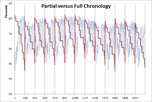 Figure 1: Partial chronology with 12 blocks per week
Fitted Chronology
 --------------------------------------------------------------------------------------------------------------------------------
 Load Slicing Settings
 --------------------------------------------------------------------------------------------------------------------------------
 Chronology..............................................................................................                  Fitted
 Step Type...............................................................................................              FISCALYEAR
 Step Count..............................................................................................                       1
 Slicing Type............................................................................................                    WEEK
 Periods per WEEK........................................................................................                      41
 Periods per Step........................................................................................                    2173
 --------------------------------------------------------------------------------------------------------------------------------
 Chronological Fitting:
 --------------------------------------------------------------------------------------------------------------------------------
 Total Time..............................................................................................                    0.13
 Convolution.............................................................................................                    0.00
 Slicing (WeightedLeastsquares)..........................................................................                    0.13
 --------------------------------------------------------------------------------------------------------------------------------
For the "Fitted" case the weighted least-squares approach is used. It ensures that the fitting of the step load function is done optimally with respect to minimizing the sum of squared errors.
In Figure 1 the duration curves are created with Block Count = 12, but the "Fitted" method is done with Block Count = 41. It is a general rule that the "Fitted" method requires a much larger number of blocks than does the "Partial" method. The number of 41 was chosen here to match approximately the number of simulation periods of the "Sampled" case below.
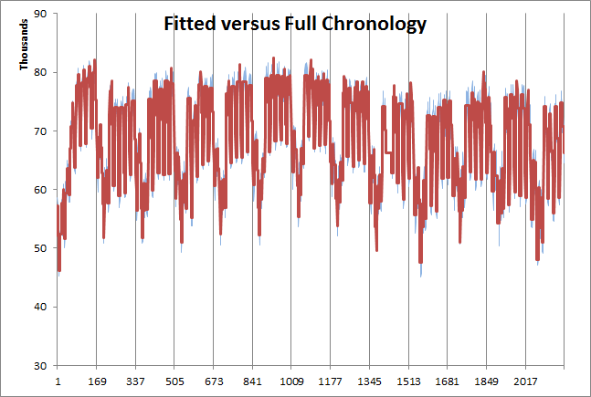 Figure 2: Fitted chronology with 41 blocks per week
In the "Partial" and "Sampled" cases, the peak load value in the month is preserved. The 'pinning' of the peak and off-peak values is controlled by the LDC Pin Top and LDC Pin Bottom settings. By default, once the number of blocks equals or exceeds seven, the peak will be 'pinned' automatically.
The additional parameters LDC Weight a, LDC Weight b, LDC Weight c, and LDC Weight d can be used to define a weighting function in the calculation of the least squares fit. The parameters define a third-order polynomial function that is used to transform the load values:
Load′ = a + b × Load + c × Load2 + d × Load3For example, from historical information you know both Load and Price. You might want to bias the slicing algorithm into putting more detail into periods of high Cost to Load. The polynomial then would represent the regression of Cost to Load to Load.
Sampled Chronology
Typical log output for the "Sampled" case is:
 --------------------------------------------------------------------------------------------------------------------------------
 Period Sampling Settings
 --------------------------------------------------------------------------------------------------------------------------------
 Sample Type.............................................................................................                    WEEK
 Sample Count............................................................................................                      53
 Reduced Sample Count....................................................................................                      13
 Relative Accuracy.......................................................................................                       1
 Sample Averaging........................................................................................                   False
 Step Count..............................................................................................                       1
 Step Length (years).....................................................................................                       1
 Step Overlap (years)....................................................................................                       0
 Periods per Step........................................................................................                    2184
 Period Sampling:
 --------------------------------------------------------------------------------------------------------------------------------
 Total Time..............................................................................................                    0.31
 Convolution.............................................................................................                       0
 Reduction...............................................................................................                       0
 --------------------------------------------------------------------------------------------------------------------------------
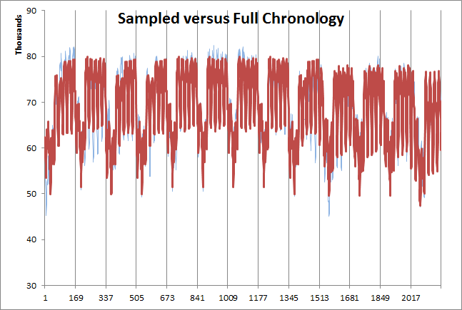 Figure 3: Sampled chronology with 13 weekly samples per year
4. Decomposition
The simulator performs the decomposition in a phase called the "MT -> ST Schedule Bridge" directly after MT Schedule.
Example
The following is typical screen output of the MT -> ST Schedule Bridge:
 MT -> ST Schedule Bridge:
 -------------------------------------------------------------------------------------------------------
 Constraint  Monthly Limit......................................................              Decomposed
 Constraint  Year # of Starts...................................................              Decomposed
 Constraint  Yearly Energy......................................................              Decomposed
 Constraint  GenMaxCapFac_Carson Peaker_month...................................              Decomposed
 Constraint  GenMaxCapFac_McClellan_month.......................................              Decomposed
 Constraint  GenMaxCapFac_PG Peaker_month.......................................              Decomposed
 -------------------------------------------------------------------------------------------------------
 Storage     Large Storage......................................................                 Targets
 Storage     Small Storage......................................................             Reoptimized
 Storage     Large Pumped Storage Head..........................................                 Targets
 Storage     Large Pumped Storage Tail..........................................                 Targets
 -------------------------------------------------------------------------------------------------------
 MT -> ST Schedule Bridge Completed. Time: 0:00:00.000
There are two types of decomposition listed here. Firstly a section dealing with Constraint objects including automatically-generated constraints resulting from the definition of properties like Generator Max Capacity Factor Month, as in the above example on the "Carson Peaker" generator. Secondly there is the Storage section which provides details on what, if any, information is being passed from MT Schedule to help co-ordinate the storage management in ST Schedule.
4.1. Constraints
MT Schedule automatically decides which Constraint objects and implied constraints such as Generator Max Energy Year need decomposition. If the constraint period is longer than the step length of ST Schedule then the constraint gets decomposed. The decomposition method can be switched between "Quantity" and "Price" modes with the setting Decomposition Method. The default is to decompose as quantities. For example a maximum energy constraint will be decomposed into an energy allocation for each day/week of ST Schedule. The allocation can be reported through the Constraint Decomposition diagnostic. A particular challenge is the handling of constraints that are slack or violated in MT Schedule. Refer to the Constraint topic for more information on the decomposition algorithm.
Should ST Schedule under or over-use the allocated quantities in any step, then 'roll over' logic keeps track of this to ensure that the original constraint is satisfied. The rollover procedure can be inspected with the Constraint Rollover diagnostic.
Note that the LDC method does not model generator start up, but start modelling is required to correctly account for Fuel usage and Emission or Max Starts constraints spanning over the medium term. Thus the LDC method might not be appropriate for modelling these constraints when starts and/or start fuel use is a significant factor. The Chronological method should be used in this case.
4.2. Hydro Storage
The bridge algorithm reports the decision taken for each Storage object out of the following options:
- Targets
The Storage End Volume from MT Schedule is to used to create a set of targets for the End Volume of each ST Schedule day or week. The target constraints are 'soft' with a penalty function described in the Storage Decomposition Method topic.
- Reoptimize
-
This means that MT Schedule decided not to decompose the storage. It might be a pumped storage that has a very small head storage for example. The storage will be freely reoptimized by ST Schedule.
- Water Value
Water left in storage at the end of each ST Schedule step is priced at the Shadow Price computed by MT Schedule.
The default choice for decomposition method can generally be over-ridden by changing the Storage Decomposition Method setting.
The results of the decomposition can be written to text files for later use in other simulations with the option Write Bridge Text Files.
5. Monte Carlo and Stochastic Simulation
MT Schedule supports multi-sample simulation, where the samples vary in the pattern of Generator and Line maintenance and/or forced outages and/or in the sample values of the stochastic Variables. By default only a single 'Expected Value' sample is run, but this can be changed with the Stochastic Method setting.
Note that the sample size for outages and stochastic sampling is set by the Stochastic object settings associated with the executing Model.
5.1. Stochastic Method
When MT Schedule is running in multi-sample mode Stochastic Method is set to "Independent Samples" or "Scenario-wise Decomposition", Constraint decomposition is performed for each sample. You should set the ST Schedule Stochastic Method setting appropriately e.g. if MT Schedule is running multi-sample then it is natural that ST Schedule should also run multi-sample.
When running in "Scenario-wise Decomposition" mode MT Schedule can perform a two-stage stochastic decomposition of Storage. See the topic Storage Trajectory Non-anticipativity for details.
5.2. Forced Outages
Similarly to LT Plan MT Schedule offers two approaches to modelling of random (forced) outages:
- Monte Carlo Simulation: Each independent sample models a unique pattern of random outages. In order to gain convergence of estimates with a high degree of confidence it is necessary to run a large number of samples. This is especially true of simulation outcomes that are sensitive to random outages such as estimates of Unserved Energy or the Price Received by peaking plant.
- Effective Load Approach: In this method the Generator Forced Outage Rate is convolved into the Region Load to produce an "Effective Load". For a description of convolution read the LOLP topic and for more details of the Effective Load Approach refer to the LT Plan documentation.
6. Capacity Expansion
MT Schedule includes an algorithm for automatic expansion of Region Generation Capacity. The algorithm is different to LT Plan and is designed for 'quick and dirty' expansion analysis.The New Entry Driver setting toggles on/off the algorithm. Only expansion of the generation side is supported, not retirements or expansion of the transmission system. These capabilities are instead available with LT Plan.
The new entry algorithm works by evaluating, at each simulation step of MT Schedule i.e. each year, whether or not one or more of the nominated potential new generation projects are economic given the simulated energy Price in the year, or if the Capacity Reserves have fallen below the required minimum such and capacity must be added for reliability purposes. The New Entry Driver setting controls whether or not reliability and/or entrepreneurial entry is considered.
6.1. New Entry Candidates
The candidate projects are identified by defining Generator Max Units Built. You should also define Generator FO&M Charge and annuities via the Equity Charge and Debt Charge (refer to LT Plan for a discussion of annuity calculations).
Example
The following tables provide examples of definitions for generic "CCGT", "GT" and "Wind" new entry candidates. Note that it is assumed the thermal generators are associated with one or more Fuels not shown here.
| Generator | Property | Value | Units | Band |
|---|---|---|---|---|
| NEW CCGT | Units | 0 | - | 1 |
| NEW CCGT | Max Capacity | 250 | MW | 1 |
| NEW CCGT | Min Stable Level | 100 | MW | 1 |
| NEW CCGT | Heat Rate | 7.7 | GJ/MWh | 1 |
| NEW CCGT | Start Cost | 1500 | $ | 1 |
| NEW CCGT | FO&M Charge | 9 | $/kW/year | 1 |
| NEW CCGT | Equity Charge | 27.75 | $/kW/year | 1 |
| NEW CCGT | Debt Charge | 45.33 | $/kW/year | 1 |
| NEW CCGT | Maintenance Rate | 10 | % | 1 |
| NEW CCGT | Forced Outage Rate | 10 | % | 2 |
| NEW CCGT | Mean Time to Repair | 36 | hrs | 1 |
| NEW CCGT | Mean Time to Repair | 6 | hrs | 2 |
| NEW CCGT | Max Units Built | 2 | - | 1 |
| Generator | Property | Value | Units | Band |
|---|---|---|---|---|
| NEW GT | Units | 0 | - | 1 |
| NEW GT | Max Capacity | 100 | MW | 1 |
| NEW GT | Min Stable Level | 20 | MW | 1 |
| NEW GT | Heat Rate | 12 | GJ/MWh | 1 |
| NEW GT | Start Cost | 500 | $ | 1 |
| NEW GT | FO&M Charge | 10 | $/kW/year | 1 |
| NEW GT | Equity Charge | 13.5 | $/kW/year | 1 |
| NEW GT | Debt Charge | 22 | $/kW/year | 1 |
| NEW GT | Maintenance Rate | 10 | % | 1 |
| NEW GT | Forced Outage Rate | 10 | % | 2 |
| NEW GT | Mean Time to Repair | 36 | hrs | 1 |
| NEW GT | Mean Time to Repair | 6 | hrs | 2 |
| NEW GT | Max Units Built | 6 | - | 1 |
| Generator | Property | Value | Units | Band | Date From | Date To | Timeslice | Data File |
|---|---|---|---|---|---|---|---|---|
| NEW WIND | Units | 0 | - | 1 | ||||
| NEW WIND | Max Capacity | 10 | MW | 1 | ||||
| NEW WIND | Rating Factor | 0 | % | 1 | CSV Files\NEW WIND.csv | |||
| NEW WIND | FO&M Charge | 4 | $/kW/year | 1 | ||||
| NEW WIND | Equity Charge | 135 | $/kW/year | 1 | ||||
| NEW WIND | Debt Charge | 220 | $/kW/year | 1 | ||||
| NEW WIND | Firm Capacity | 0.8 | MW | 1 | ||||
| NEW WIND | Max Units Built | 50 | - | 1 |
6.2. New Entry Algorithm
For entrepreneurial entry, the simulator calculates the premium (over variable costs) that each of the candidate generators would receive given the MT Schedule price duration curve for the year ahead. For reliability entry, the candidate with the highest premium (even if a loss is implied) will be entered. If entrepreneurial entry is considered, the same premia are used to select potentially profitable new entrants. Units are entered one-by-one, and the price duration curve is adjusted appropriately each time, so the premium for each candidate reduces as new units are added until eventually no more plant can be profitably entered.
This approach is very similar to that which would be used by an entrepreneur calculating the profitability of potential projects except that MT Schedule only looks one year ahead, and assumes that all future years will be the same. Thus this method only approximates optimal entrepreneurial entry.
Capacity entered to meet reliability criteria is always entered at the beginning of the MT Schedule step in which it is required e.g. if a capacity shortfall were forecast to occur in February, and the horizon steps through calendar years, then the new generator will begin operation on January 1 of the year it. By default new entrepreneurial generators will begin operation in the year immediately following their selection. This behaviour can be controlled with the New Entry Time Lag setting.
Example
With New Entry Driver set to "Entrepreneurial Only" the following report appears in the log during execution. It details firstly the peak load period and how much Generation Capacity is available at that time. Net Capacity Interchange is reported and the resulting Capacity Reserves. The next section listed the new entry candidates and their:
- Rated Capacity (MW)
- The average megawatt Rating of the generator in the year.
- Firm Capacity (MW)
- The Firm Capacity of the generator at the period of Peak Load. This is the contribution the Generator makes to Capacity Reserves.
- Variable Cost ($/MWh)
- The SRMC at Max Capacity accounting for the incremental cost of emissions.
- Required Premium ($/kW/year)
- The total fixed cost charge the Generator must recover in order to break-even.
- Available Premium ($/kW/year)
- How much profit one generating unit of the Generator would make given the current price duration curve.
 Entrepreneurial Expansion:

 -------------------------------------------------------------------------------------------------------
 SA Capacity
 -------------------------------------------------------------------------------------------------------
 Peak Load (Friday, 21 January 2011)........................................................     3530.00
 Required Capacity Reserves.................................................................        NONE
 Required Capacity Reserve Margin...........................................................        NONE
 Firm Generation Capacity...................................................................     3692.50
 Net Capacity Interchange...................................................................     -660.00
 Capacity Reserve...........................................................................      822.50
 Capacity Reserve Margin....................................................................     23.30 %
 Capacity Reserve Deficit...................................................................        0.00

 Pass 1
 -------------------------------------------------------------------------------------------------------
 Generator                                    Rated       Firm        Variable    Required    Available
                                              Capacity    Capacity    Cost        Premium     Premium
                                              (MW)        (MW)        ($/MWh)     ($/kW/yr)   ($/kW/yr)
 -------------------------------------------------------------------------------------------------------
 NEW CCGT...................................      250.00      250.00       30.80       82.08       49.12
 NEW GT.....................................      100.00      100.00       48.00       45.50       42.29
 NEW WIND...................................        3.01        0.80        0.00      359.00      355.74
 -------------------------------------------------------------------------------------------------------
 Entrepreneurial Expansion Completed
The Available Premium must be large enough to cover the Required Premium for the given new entrant to be selected. If it is selected a message like the following is printed to the log and the entry is labelled with Status of "Entrepreneurial":
 Generator Added                                                       Capacity    Status
 -------------------------------------------------------------------------------------------------------
 NEW WIND...........................................................        3.02         Entrepreneurial
Generators added to maintain the required Min Capacity Reserves be are listed in the log file as in the following example with Status of "Reliability". The candidate with the highest premium is selected.
 -------------------------------------------------------------------------------------------------------
 Generator                                    Rated       Firm        Variable    Required    Available
                                              Capacity    Capacity    Cost        Premium     Premium
                                              (MW)        (MW)        ($/MWh)     ($/kW/yr)   ($/kW/yr)
 -------------------------------------------------------------------------------------------------------
 NEW CCGT...................................      250.00      250.00       30.80       82.08       50.14
 NEW GT.....................................      100.00      100.00       48.01       45.50       39.12
 -------------------------------------------------------------------------------------------------------
 Generator Added                                                      Capacity    Status
 -------------------------------------------------------------------------------------------------------
 NEW GT.............................................................      100.00             Reliability
 -------------------------------------------------------------------------------------------------------
Addition of capacity continues each year to meet the required reserves and/or when profitable as set the New Entry Driver.
Figures 4-7 show example results from simulations with New Entry Driver = "Entrepreneurial Only". Figures 8-11 repeat those for New Entry Driver = "Reliability and/or Entrepreneurial".
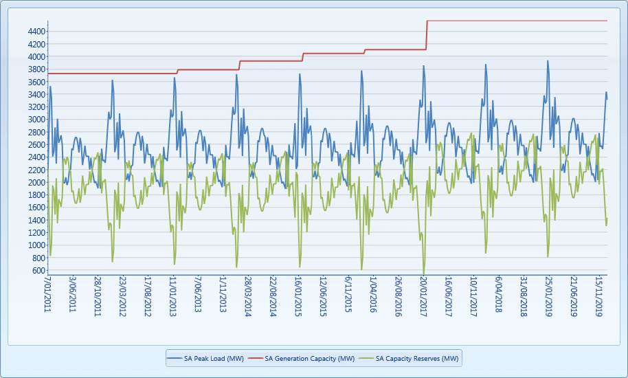 Figure 4: Region Capacity Balance (Entrepreneurial Only)
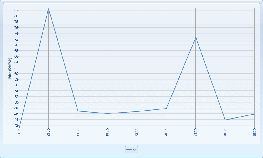 Figure 5: Region Price (Entrepreneurial Only)
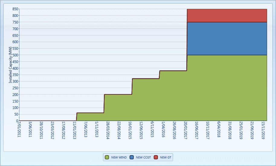 Figure 6: New Entrant Capacity (Entrepreneurial Only)
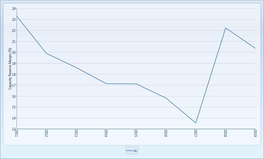 Figure 7: Region Capacity Reserve Margin (Entrepreneurial Only)
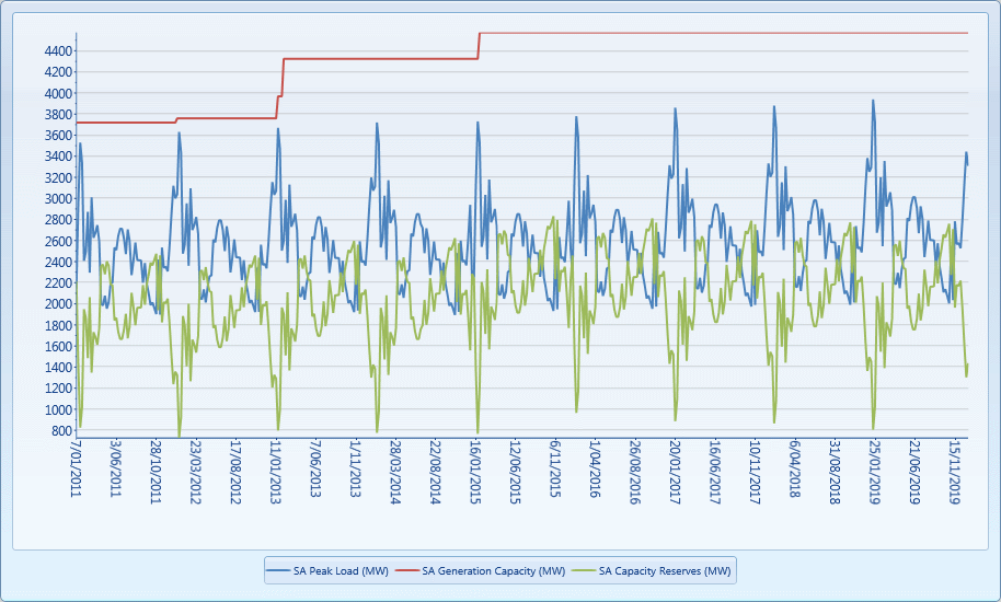 Figure 8: Region Capacity Balance (Reliability and
Entrepreneurial 20% Min Capacity Reserve Margin)
Figure 8: Region Capacity Balance (Reliability and
Entrepreneurial 20% Min Capacity Reserve Margin)
 Figure 9: Region Price (Reliability and Entrepreneurial 20% Min
Capacity Reserve Margin)
Figure 9: Region Price (Reliability and Entrepreneurial 20% Min
Capacity Reserve Margin)
 Figure 10: New Entrant Capacity (Reliability and
Entrepreneurial 20% Min Capacity Reserve Margin)
Figure 10: New Entrant Capacity (Reliability and
Entrepreneurial 20% Min Capacity Reserve Margin)
 Figure 11: Region Capacity Reserve Margin (Reliability and
Entrepreneurial 20% Min Capacity Reserve Margin)
Figure 11: Region Capacity Reserve Margin (Reliability and
Entrepreneurial 20% Min Capacity Reserve Margin)