Variable Class
| Description: | Stochastic variable |
See also Variable Property Reference for a detailed list of properties for this class of object.
- Introduction
- Conditional Variables
- Escalator Variables
- Stochastic Variables
- Machine Learning Models
1. Introduction
The variable class can be broadly categorized into three different types. These are:
- Conditional Variables - variables which are used to activate/deactivate other objects or properties based on certain conditions that occur in the simulation.
- Escalator Variables - variables which are used to automatically change a datum over time according to the value of a user-defined index.
- Stochastic Variables - variables which define stochastic or expected profile data.
2. Conditional Variables
Conditional Variable objects are used to activate/deactivate other objects or properties based on certain conditions that occur in the simulation. Conditions can be applied to Constraints and to Financial Contracts.
The property Profile is used as a flag that indicates if the condition is active in any given period. It can take the following values:
- value = -1
- - Condition is active.
- value = 0
- - Condition is inactive.
Note: The Variable Sampling Method attribute must be set to "None" to be considered as a conditional variable.
2.1. Static Conditional Variables
In the simplest case the Profile property can be set statically, for example:
| Variable | Property | Value | Units | Timeslice |
|---|---|---|---|---|
| PEAK | Profile | -1 | - | PEAK |
| SUMMER PEAK | Profile | -1 | - | SUMMER, PEAK |
Here the Variable "PEAK" is active according to the definition of the "PEAK" Timeslice, and the variable "SUMMER PEAK" is active only when both the PEAK and SUMMER timeslices coincide.
The Profile property can be input like any other PLEXOS input e.g. set using dates and time, patterns (timeslices), or even read from a text file.
2.2. Dynamic Conditional Variables
A dynamic conditional variable is one whose 'sample' Value must be determined during the simulation because it is dependent on one or more simulation variables.
A dynamic conditional variable is defined like an equation. It has a left-hand side of terms, a sense, and a right-hand side. The equation is evaluated in every period to see if the variable condition should be active in the period:
Conditional Variable "is active" if Left-hand Side (≤, =, ≥) Right-hand SideThe simulator uses the same numeric code for the variable condition (sense) as for the sense of Constraints and exposes many of the same left-hand side variables as for Constraints.
Example
| Variable | Property | Value | Units |
|---|---|---|---|
| TORRB | Condition | 1 | - |
| TORRB | Profile | 2 | - |
| Variable | Generators | Property | Value | Units |
|---|---|---|---|---|
| TORRB | TORRB1 | Units Generating Coefficient | 1 | - |
| TORRB | TORRB2 | Units Generating Coefficient | 1 | - |
| TORRB | TORRB3 | Units Generating Coefficient | 1 | - |
| TORRB | TORRB4 | Units Generating Coefficient | 1 | - |
In this example the variable is active only when two or more units are committed (on-line) at the specified power station. Specifically the conditional variable as defined says:
Conditional Variable ( TORRB ) Is Active if: TORRB1.UnitsCommited + TORRB2.UnitsCommited + TORRB3.UnitsCommited + TORRB4.UnitsCommited ≥ 2Most conditional variables involve summing variables e.g. megawatts of demand, or transmission flows, or unit committed at a power station and testing the result against some right-hand side value, but there are some special cases where the left-hand side coefficient returns a logical (0, -1) value itself that can be directly tested for. An example is the direction of flow on a transmission line, which can be tested using the Flowing Forward and Coefficient properties.
The output Value for the Variable corresponds to the result (true/false) of the conditional expression, while Activity reports the sum of the left-hand side of the conditional expression that is compared against Profile according to the Condition type.
2.3. Applying Conditional Variables
You can apply conditions to:
- Constraints to create conditional constraints.
- Financial Contracts to create contracts that only activate in particular circumstances.
- Properties to make the property conditional (using the Variable and Action fields in the Property Grid).
- Make the value of one Variable to equal the left-hand side (Activity) of another Variable by assigning the conditional variable you want the LHS value from as a condition membership , set the Activity Coefficient to 1, and the Profile to zero, then assign the variable where needed.
- Simply use a conditional Variable to report a calculated values based on the Activity.
Example
| Generator | Property | Value | Units | Action | Expression |
|---|---|---|---|---|---|
| G1 | Rating | 200 | MW | ||
| G1 | Rating | 220 | MW | ? | G3 OOS |
Here the Generator G1 normally has a rating of 200 MW but can boost this to 220 MW when the "G3 OOS" variable condition is active.
2.4. Combining and Nesting Conditional Variables
There are two ways you can combine conditions to form more complex logic:
- You can combine conditions in the expression property field in the same way that you can combine Timeslices.
- You can nest conditions by making a condition the product or multiple other conditions.
2.4.1. Combining Conditional Variables
Example
| Constraint | Property | Value | Units | Action | Expression |
|---|---|---|---|---|---|
| X-Y | RHS | 1400 | MW | ||
| X-Y | RHS | 1550 | MW | ? | G1 OOS, G2 LT 300 |
In this example the RHS property for the constraint is 1400, except if both the conditional variables "G1 OOS" AND "G2 LT 300" are both active, and then the limit is 1550.
2.4.2. Nesting Conditional Variables
Another way to combine conditions is to nest them by creating a condition that is the product of two or more other conditions. This is achieved by adding elements into the Conditions collection of the condition. You can then decide whether those conditions are combined using AND or OR logic using the Condition Logic property.
Note that if you create a condition as the product of other conditions you cannot set Is Active or define a dynamic equation for that condition. Also you can only nest conditions one level deep i.e. a condition cannot be conditional on other conditional conditions.
2.5. Conditional Variables For Look-ahead Patterns
Defining timeslice patterns for look-ahead periods is achieved by defining a special kind of conditional variable. This variable should have no memberships defined, condition = none, profile = 0, no sampling properties defined, and the look-ahead pattern set on profile. Only one look-ahead pattern should be defined per variable. To apply this look-ahead pattern to a property simply set the property's action to "?" and the expression to the variable. See the example below which sets the Region Load for REG to 220 MW for intervals 1 to 6 of the look-ahead.
| Variable | Property | Value | Units | Timeslice |
|---|---|---|---|---|
| LA | Profile | 0 | - | L1-6 |
| Region | Property | Value | Units | Action | Expression |
|---|---|---|---|---|---|
| REG | Load | 220 | MW | ? | LA |
Please note when modeling lookahead periods of a different resolution to the chronological horizon and pointing the lookahead periods to use a data file of type period, then the data file is interpreted as having the resolution of the chronological horizon, not the lookahead.
Some examples of valid look-ahead patterns are as follows.
| Pattern | Interpretation |
|---|---|
| L1 | Look-ahead interval one |
| L1-24 | Look-ahead intervals 1 to 24 |
| L1-12, 24 | Look-ahead intervals 1 to 12, and interval 24 |
NOTE: Applying Look-ahead patterns to properties will not work if the property is also set to equal the value of another variable.
3. Escalator Variables
Escalator Variable objects are used to automatically change a datum over time according to the value of a user-defined index. Escalator Variables are simple objects with basic input properties, such as:
- Variable Profile
- Variable Compound Index
- Variable Compound Index Day
- Variable Compound Index Hour
- Variable Compound Index Week
- Variable Compound Index Month
- Variable Compound Index Year
Note: The Variable Sampling Method attribute must be set to "None" to be considered as an escalator variable.
3.1. Applying Escalator Variables
The Profile property can act as an "index" or "scalar" value. For example, the following shows a variable called "CPI" and its application to a fuel price. The example shows how a 3% compounding escalation in fuel prices would be modelled. Note that in PLEXOS you may create as many escalators variables as you need and apply them to any input data.
Example definition of an escalator variable:
| Variable | Property | Value | Units | Date From |
|---|---|---|---|---|
| CPI | Profile | 1 | - | 1/01/2004 |
| CPI | Profile | 1.03 | - | 1/01/2005 |
| CPI | Profile | 1.0609 | - | 1/01/2006 |
| CPI | Profile | 1.092727 | - | 1/01/2007 |
Example application of the escalator to fuel prices:
| Fuel | Property | Value | Units | Action | Expression |
|---|---|---|---|---|---|
| Gas | Price | 6 | $/MMBTU | * | CPI |
In addition to this both conditional and escalated variable objects can be combined and applied to a property. For example " IsOn" has been defined as a conditional variable, while " VarIncr" has been defined an escalator variable:
| Class | Name |
| Region | Australia |
| Variable | IsOn |
| Variable | VarIncr |
| Collection | Name | Property | Value | Units | Action | Expression |
| Regions | Australia | Load | 0 | MW | ? | if( IsOn, VarIncr) |
The result of this is that the " IsOn" variable is tested for its "Active" flag and if that is true the " VarIncr" variable will be used. If " IsOn" is not true then this property will not be used, there is no "else" statement. Note that the second parameter of the "if" statement can be any variable type (excluding conditional variables).
4. Stochastic Variables
Variable objects form the foundation of the stochastic modelling. Variables are not tied to any particular element of the data model, and thus are completely generic. This means that any datum in the system can be made stochastic i.e. not just the 'usual' elements such as load, hydro and fuel price. And further, any number of variables (stochastic elements) may be included in any database - up to the limit of practicality of sampling across multiple variables.
There are two approaches for randomizing a datum:
- Directly define a set of chronological samples that can be randomly selected when sampling - these sequences can be correlated e.g. the demand in two regions may be correlated, but each can be supplied with a set of demand trances with various associated probabilities.
- Define the expected value and information on how errors are distributed and allow the simulation engine to generate the required samples.
4.1. User-defined Samples
4.1.1. Defining the Samples
In this scheme you supply the samples for the Variable. A Variable can represent any datum e.g. the Load in a Region, or the Natural Inflow to a Storage. There can be any number of samples input for any one Variable and this is done using the Profile property in multiple bands. Each sample should appear on a different band number and the band numbers should be contiguous. The Profile property can vary in the usual way i.e. by date, pattern, or read from a text file using the Data File field, and multi-band data can be read from a single text file. Multiple Data File entries can be defined with different Date From and Date To.
There are several ways in which the defined samples are used and this is controlled by the Variable Sampling Method setting and definition of Profile and other properties as follows.
4.1.2. Random Sampling
When Sampling Method = "Random Sampling" the sampling approach depends on:
- How many bands of data are defined for Profile
- Whether or not you define either Error Std Dev or Abs Error Std Dev
Single-band Profile
If Profile is defined with a single band (as in Table 1) then samples will be drawn around that profile value using it as the 'expected value' (mean). Errors will be distributed normal or lognormal depending on Distribution Type). Please note that one of the Endogenous Sampling models (See in section 4.3) should be specified with its corresponding parameters to invoke random sampling, otherwise the samples will be read directly from Profile.
Multi-band Profile
If Profile is defined with multiple bands, then one of four sampling schemes will be used depending on which other properties are defined:
- If you also define either Error Std Dev or Abs Error Std Dev then the multi-band Profile data will be averaged point-by-point and sampling will occur just as in the single-band example in Table 1
- If instead you define the Probability property (as in Table 2) the simulator generates error values from a normal or lognormal distribution (see Distribution Type) then selects the band that most closely matches the probability of the random draw in each sample. This Probability property is interpreted as the probability of exceedance of the observation e.g. a probability of 10% applied to the first band of load forecast means that the forecast demand is expected to occur no more than once in 10 samples, likewise a probability of 90% in the second band would occur no more than 9 times in 10 samples, and a probability of 80% (when given in combination only with 80% and 100% profiles) would occur in about 80% of the samples
- If none of the above definitions apply then the provided bands are selected randomly for each sample i.e. depending on the random number drawn, sample (band) one might be chosen in one sample, sample (band) three in another and so on.
A more powerful version of Option 3 is to sample the bands randomly at specific time intervals. For example you might input 12 historical years of weekly hydro inflow data and want the simulator to pick from those sequences randomly. Of course the theoretical number of combinations (samples and weeks) is enormous, but the simulator can generate a random selection of that space for you. This is achieved with the Sampling Frequency setting and the Sampling Period Type. Here you can also define either Error Std Dev or Abs Error Std Dev for the sequences. To continue you the example you could set:
- Sampling Frequency = 1 (each period type period)
- Sampling Period Type = 2 (period type is weekly)
Option 3 can also be used to study multiphase phenomena. One two-phase example is the El Nino-Southern Oscillation:
some years are distinctly 'warm' while others are 'cold'. In the following example, two Profile bands
are defined based on other Variables. The two constituent Variables add noise to historical data from
warm and cold years. The combined variable will alternate between the warm and cold modes from sample to sample.
| Variable | Property | Value | Data File | Band | Action | Expression |
|---|---|---|---|---|---|---|
| Var_El_Nino | Profile | 0 | 1 | + | Var_El_Nino_Warm | |
| Var_El_Nino | Profile | 0 | 2 | + | Var_El_Nino_Cold | |
| Var_El_Nino | Sampling Method | Auto | 1 | = | ||
| Var_El_Nino_Warm | Profile | 0 | Warm_EN_Trace | 1 | = | |
| Var_El_Nino_Warm | Error Std Dev | 20 | 1 | = | ||
| Var_El_Nino_Warm | Sampling Method | Auto | 1 | = | ||
| Var_El_Nino_Cold | Profile | 0 | Cold_EN_Trace | 1 | = | |
| Var_El_Nino_Cold | Error Std Dev | 20 | 1 | = | ||
| Var_El_Nino_Cold | Sampling Method | Auto | 1 | = |
The simulator will then draw a number of samples (set by Stochastic Risk Sample Count) and optionally reduce down to the Reduced Sample Count for simulation.
It is possible to sample any number of times against a single Variable regardless of how many bands are defined. For example, there may be three demand, and 100 hydro inflow bands supplied. In this case the three demand sequences will likely be chosen multiple times if Risk Sample Count = 100.
Examples
Table 1: Single Band Profile Random Sampling
| Property | Value | Unit | Band | Date From | Date To | Timeslice | Data File |
|---|---|---|---|---|---|---|---|
| Profile | 0 | - | 1 | Electric Price.csv | |||
| Error Std Dev | 20 | % | 1 | ||||
| Autocorrelation | 70 | % | 1 |
In this case the expected values are read from the data file "Electric Price.csv" and samples are drawn around that with error terms normally distributed and correlated in time.
Table 2: Samples in Multiple Bands with Probability
| Property | Value | Units | Band |
|---|---|---|---|
| Profile | 1 | - | 1 |
| Profile | 2 | - | 2 |
| Profile | 3 | - | 3 |
| Profile | 4 | - | 4 |
| Profile | 5 | - | 5 |
| Profile | 6 | - | 6 |
| Profile | 7 | - | 7 |
| Profile | 8 | - | 8 |
| Profile | 9 | - | 9 |
| Profile | 10 | - | 10 |
| Probability | 5 | % | 1 |
| Probability | 15 | % | 2 |
| Probability | 25 | % | 3 |
| Probability | 35 | % | 4 |
| Probability | 45 | % | 5 |
| Probability | 55 | % | 6 |
| Probability | 65 | % | 7 |
| Probability | 75 | % | 8 |
| Probability | 85 | % | 9 |
| Probability | 95 | % | 10 |
In this example the Variable takes values from one to 10, with equal probability. To illustrate, a simulation was run with Risk Sample Count = 1000 (samples). Figure 1 is a histogram of the 1000 normally distributed random numbers, and Figure 2 illustrates how many times each user-defined sample was selected - consistent with the uniformly distributed probabilities given. Figure 3 captures the chart of the property this variable applied to in the simulation when the Statistics option is chosen in the charting interface.
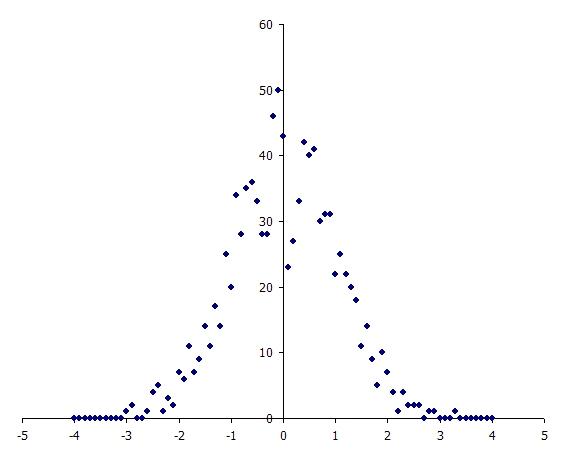 Figure 1: Normally Distributed Random Numbers
 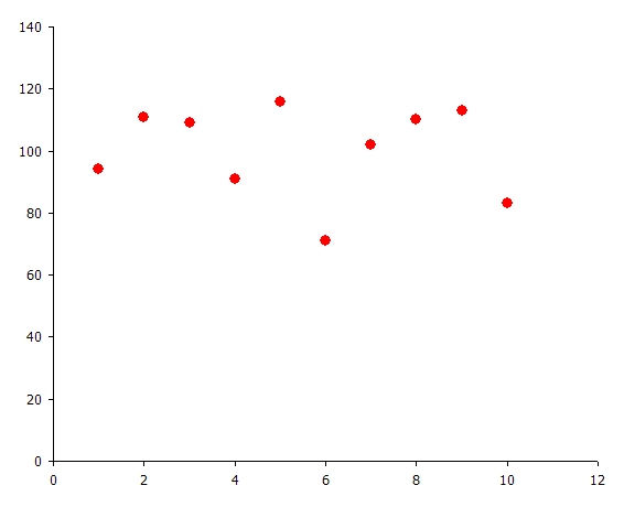 Figure 2: Frequency of Sample Selection
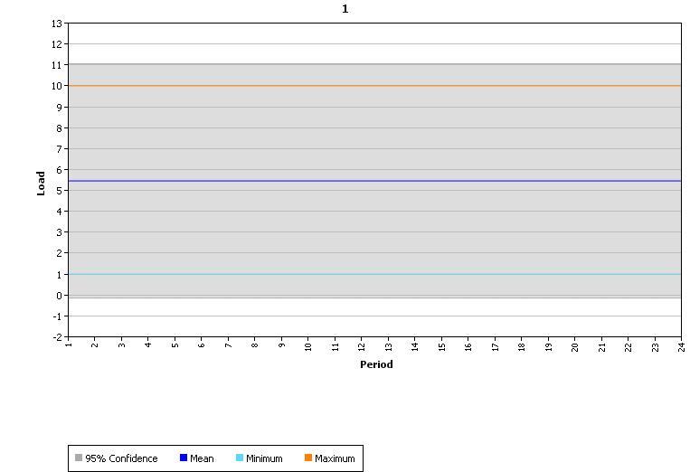 Figure
3: Statistics and Confidence Interval
Figure
3: Statistics and Confidence Interval
4.1.3. Samples in Bands
When Sampling Method = "Samples in Bands" samples in the simulation ( Stochastic Risk Sample Count) are matched against the user-defined sample bands one-to-one. Band 1 of Profile is used for sample 1, band 2 for sample 2 and so on. The Variable Probability is not used in this scheme. This scheme is useful when performing selective sampling.
4.1.4. Historical Sampling
When Sampling Method = "Samples in Bands" (i.e. "User") samples in the simulation, a historical Sampling can be defined by enabling the Data file Attribute Historical Sampling. There should be only one historical sample input for the Variable and the historical data will be mapped into the Profile property with multiple bands by using a predefined mapping scheme. This scheme is particularly designed to work for constructing scenario tree with hanging branches.
4.2. Selective Sampling and Sample Weights
The number of samples run in the simulation is controlled by the Stochastic Risk Sample Count settingcall this S, the sample count. By default the 'weight' w s applied to each of the S samples is uniform. Thus the simulator calculates the expected value of an output as a weighted-average based on these (uniform) weights. In stochastic optimization (see Stochastic Method for example) the objective function of the simulation contains all S samples weighted by these w s .
Because the weights are uniform you must use a large sample size to obtain estimates of these expected values with a reasonable degree of certainty
4.2.1. Selective Sampling
A method often used to reduce the required sample size is 'selective sampling'. In this scheme the weights of the samples are not uniform and the samples are chosen deliberately to cover a range of possibilities but with low weighting given to extreme sample values.
Example
Assume that we have a Variable whose probability distribution is normal with μ = 500 and σ = 20%. We could define this as follows:
| Property | Value | Units | Band |
|---|---|---|---|
| Sampling Method | "Random Sampling" | - | 1 |
| Profile | 500 | - | 1 |
| Error Std Dev | 20 | % | 1 |
| Min Value | 0 | - | 1 |
| Max Value | 1000 | - | 1 |
| Auto Correlation | 0 | % | 1 |
We could now run with S = 1000 and the simulator will select values according to the normal distribution. Figure 4 shows a histogram of the resulting sample values.
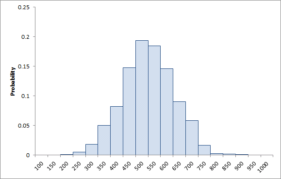 Figure 4:Histogram of 1000 samples
To implement selective sampling here you can define your (limited set of) samples using multi-band Profile properties as in the following example where five samples are defined:
| Property | Value | Units | Band |
|---|---|---|---|
| Sampling Method | "Samples in Bands" | - | 1 |
| Profile | 250 | - | 1 |
| Profile | 350 | - | 2 |
| Profile | 500 | - | 3 |
| Profile | 650 | - | 4 |
| Profile | 750 | - | 5 |
Sampling Method is set to "Samples in Bands" to indicate that the samples should be matched against the S simulation samples one-to-one. It remains only to over-ride the uniform weights applied to the samples by the simulator so that we achieve weights like that shown in Figure 5.
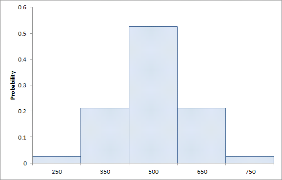 Figure 5:Selective Sampling of Normally Distributed Variable
4.2.2. Sample Weights
Whether or not you are performing selective sampling you can control the weight applied to samples in the simulation. There are two methods for input of sample weights:
- By defining a Global object with property Sample Weight in multiple bands (PLEXOS Version 6.3 and above.
- By defining the sample weights in a XML parameter file.
For the second method, the sample weights ( w s ) are input via a special parameters XML file called "PLEXOS_Param.xml". This text file has the following content for this example:
<?xml version="1.0" standalone="yes"?>
 <UndocumentedParam xmlns="http://tempuri.org/UndocumentedParam.xsd">

   <Stochastic>
     <ParameterName> SampleWeightingMethod </ParameterName>
     <Value> 1 </Value>
   </Stochastic>

   <Stochastic>
     <ParameterName> SampleWeight </ParameterName>
     <Value> 0.025 </Value>
     <Band> 1 </Band>
   </Stochastic>

   <Stochastic>
     <ParameterName> SampleWeight </ParameterName>
     <Value> 0.2125 </Value>
     <Band> 2 </Band>
   </Stochastic>

   <Stochastic>
     <ParameterName> SampleWeight </ParameterName>
     <Value> 0.525 </Value>
     <Band> 3 </Band>
   </Stochastic>

   <Stochastic>
     <ParameterName> SampleWeight </ParameterName>
     <Value> 0.2125 </Value>
     <Band> 4 </Band>
   </Stochastic>

  <Stochastic>
    <ParameterName> SampleWeight </ParameterName>
    <Value> 0.025 </Value>
    <Band> 5 </Band>
  </Stochastic>

 </UndocumentedParam>
The parameter " SampleWeightingMethod" can take these values:
- "Uniform" (default, value = 0)
- Samples in the simulation are weighted uniformly.
- "Custom" (value = 1)
- Sample weights are user-defined and read from the " SampleWeight" parameters where the Band field represents the sample number.
The Stochastic Risk Sample Count is now set to 5 ( S = 5).
4.3. Endogenous Sampling
Each Variable object represents a chronological stream of data. In the endogenous sampling scheme, the data has an expected value which may vary period-to-period as in a load forecast or may vary month-to-month as in a hydro energy budget or any other pattern as required (daily, weekly, monthly, annual). The Variable property Profile sets the expected value for the stochastic variable. The Profile property accepts all the usual methods of input including use of the Data File field to read the data from a text file, or it can point to a Data File object. In this case however, only one band is used for the Profile property.
A variable object should contain data for one period type only and this period type is dictated by which Profile property is set ( Profile, Profile Hour, Profile Day, Profile Week, Profile Month, or Profile Year). For example, a load forecast would use the Profile property meaning that the stochastic variable changes on a period-by-period basis, but a monthly hydro energy budget would use Profile Month.
You can freely mix the sampling frequency with the type of data the Variable is applied to. For example you might define Profile Month to draw random Fuel Price values on a monthly basis.
By default the simulator will randomly generate 'errors' around the expected profile value for each Variable. The shape of the error distribution may be either normal or lognormal as set by the Distribution Type property.
Note: If you prefer to specify some precomputed or historical profiles, the Profile property is allowed to be multi-band i.e. a number of different profiles can be specified along with their associated probabilities: see above.Each stochastic variable 'works' by applying a differential equation to create an error function across time. These errors represent random variations around the expected value. There are three methods available:
- Simple autocorrelation
- Brownian motion with mean reversion
- Box-Jenkins method
The following models can be used for Box-Jenkins method:
- ARMA - Autoregressive moving average model
- ARIMA - Autoregressive integrated moving average model
The method that will be used is determined by one of the input parameters of the corresponding method. For example, if the input parameter ARIMA α (or ARIMA β) is set the Box-Jenkins method will be used, and if the input parameter Mean Reversion is set the Brownian motion method will be used. More details can be found in the following sections.
4.3.1. Autocorrelation Model
In the autocorrelation model, the differential equation is:
The input parameters here are the Autocorrelation and the Error Std Dev (alternatively Abs Error Std Dev. Autocorrelation is expressed as percentage value (between 0 and 100). The higher the autocorrelation, the more the 'randomness' of the errors is dampened and smoothed out over time. The higher the standard deviation, the greater the volatility of the errors. Because the error function can produce any positive or negative value (at least in theory) it is often necessary to bound the profile sample values produced by this method. The Variable properties Min Value and Max Value are used for this purpose. The actual sample value used at any time is simply the sum of the profile value and the error (which may be positive or negative) bounded by the min and max values.
Table 2 shows some simple example input where the profile value is static but has an error function with standard deviation of 28%. In a real application the profile value would change across time e.g. read from a flat file. Figure 6 shows the resulting distribution of sample values from 1000 samples, which follows a normal distribution. Figures 7 and 8 shows the output sample 1 profiles with the autocorrelation parameter set to 0% and 75% respectively. Note that the overall distribution of the sample values is still normal as in Figure 6, but the individual sample volatility is damped.
| Property | Value | Units | Band |
|---|---|---|---|
| Profile | 5.5 | - | 1 |
| Error Std Dev | 28 | % | 1 |
| Min Value | 1 | - | 1 |
| Max Value | 10 | - | 1 |
| Auto Correlation | 75 | % | 1 |
Table 2: Sampling with Autocorrelation
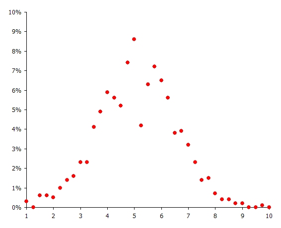 Figure 6: Histogram of Sample Values
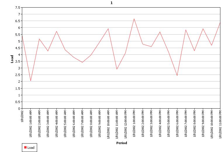 Figure
7: Sample 1 Profile with No Autocorrelation
Figure
7: Sample 1 Profile with No Autocorrelation
 Figure
8: Sample 1 Profile with 75% Autocorrelation
Figure
8: Sample 1 Profile with 75% Autocorrelation
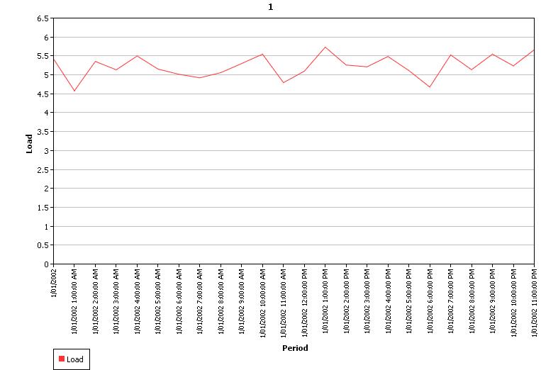
4.3.2. Mean Reversion Models
4.3.2.1. Brownian Motion with Mean Reversion
In this model, the differential equation is:
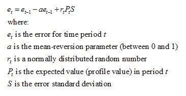
Table 3 shows some example input for this case. Figure 9 shows the sample 1 profile with a mean reversion parameter of 0.75.
| Property | Value | Units | Band |
|---|---|---|---|
| Profile | 5.5 | - | 1 |
| Error Std Dev | 28 | % | 1 |
| Min Value | 1 | - | 1 |
| Max Value | 10 | - | 1 |
| Mean Reversion | 0.1 | - | 1 |
Table 3: Sampling with Mean Reversion
 Figure 9: Sample 1 Profile with Mean Reversion of 0.75
4.3.2.2. Jump Diffusion with Mean Reversion
In this model, the differential equation is:
If the jump frequency, jump magnitude and jump standard deviation are all provided, the jump term will be added to the Brownian Motion with Mean Reversion, i.e, using the Jump Diffusion with Mean Reversion model.
Notice:
- The jump frequency is the number of jumps per year (assume 365 days a year). The number of jumps per period should be a value much smaller than 1.0, otherwise the resolution is too low.
- The jump magnitude is the ratio of the sample values with and without jumps.
4.3.3. Box-Jenkins method
4.3.3.1. ARMA model
This model consists of two parts, an autoregressive (AR) part and a moving average (MA) part.
- AR(p) model
The autoregressive part of order p is defined by p autoregressive parameters ARIMA α, where the differential equation is defined by:
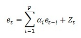
where:
et is the error for the time period t
α1,...,αp are the autoregressive
parameters ARIMA α
Zt is a normally distributed number with standard
deviation of σ for the time period t
- MA(q) model
The moving average part of order q is defined by q moving average ARIMA β, where the differential equation is defined by:
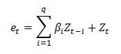
where:
et is the error for the time period t
β1,...,βq are the moving average
parameters ARIMA β
Zt is a normally distributed number with standard
deviation of σ for the time period t
- ARMA(p,q) model
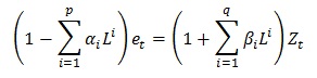
Hence, ARMA(p,q) refers to a model with p autoregressive terms and q moving average terms, where the differential equation is defined by:
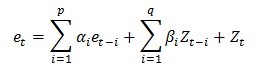
where:
et is the error for the time period t
α1,...,αp are the autoregressive
parameters ARIMA α
β1,...,βq are the moving average
parameters ARIMA β
Zt is a normally distributed number with standard
deviation of σ for the time period t
Using the lag operator L, where:
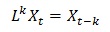
ARMA(p,q) can expressed in terms of the lag operator L, where:
4.3.3.2. ARIMA model
This model is a generalisation of an ARMA model, where an integrated part is introduced. The ARIMA(p,q,d) differential equation is defined by:
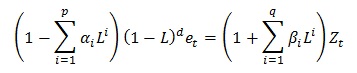
d is the differencing parameter ARIMA d
4.4. Volatility Metric
EWMA (Exponential weighted moving average) and GARCH (generalized autoregressive conditional heteroskedasticity) models allow for the modeling of volatility clustering.
In the EWMA case, the differential equation is:
σ 2( t) = (1 - λ) r 2( t-1) + λ σ 2( t-1)where:
λ is the coefficient of decayr(t) is return in period t, r(t) = [P(t) - P(t-1)] / P(t-1)
σ(t) is the volatility for time period t
In the GARCH (1,1) case, the differential equation is:
σ 2( t) = ω + α r 2( t-1) + β σ 2( t-1)where:
ω is the long-run weighted varianceα, β are the weights on the square of the return and the variance, respectively
r(t) is return in period t, r(t) = [P(t) - P(t-1)] / P(t-1)
σ(t) is the volatility for time period t
Note that if ω is assumed to be 0 and α+ β is assumed to be 1, then the GARCH model becomes identical to the EWMA model.
4.5. Sample Tree Tool
4.5.1. Sample Reduction
In practice, the optimization problem that contains all possible scenarios (the stochastic samples) is too large. To decrease the challenge of computational complexity and time limitations in optimization, the original problem is often approximated by a model with a much smaller number of samples. The Sample Reduction algorithm is developed to reduce the number of samples to a predefined smaller number but with the reduced samples being still a good approximation of the original problem. The reduction is based on rules that ensure only the samples that are similar to other samples or have small probabilities will be combined.
The input parameter for the Sample Reduction algorithm is Reduced Sample Count (how many samples to be preserved), or Reduction Relative Accuracy (how much information to be preserved). The default value for Reduced Sample Count is zero, which means no sample will be reduced. The value for Reduction Relative Accuracy should be between 0 and 1, which are corresponding to reduction with only one sample to be preserved and no reduction, respectively. For sample reduction, at least one of the parameters should be provided. If both parameters are available, the reduction process will be stopped only when both conditions are satisfied.
For example, there are a set of samples with Sample Count = 20, and the Reduction Relative Accuracy = 0.63 if the samples are reduced to 10. To make the expected sample reduction, we can set Reduced Sample Count = 10, or Reduction Relative Accuracy = 0.63. If we set Reduced Sample Count = 12 and Reduction Relative Accuracy = 0.63, the number of samples will still be reduced to 10, since the latter criterion must also be satisfied.
If only Reduced Sample Count is provided, the algorithm described in [1] is used, otherwise we use the one based on the relative accuracy which is detailed in [2]. Notice that, in order to decrease the reduction time for samples with a very large Sample Count, we have changed the distance calculation method from the 2-norm [\sqrt{\sum_{i=1}^{n} (s1_i-s2_i)^2}] to the 1-norm [\sum_{i=1}^{n} \abs(s1_i-s2_i)], where s1_i and s2_i are the values of sample 1 and sample 2 at position i, respectively. More information on this topic can be found in the two papers and other relevant references.
Controlling parameters:
4.5.2. Sample Tree Construction
In multi-stage stochastic programming models, such as in Hydro Reservoirs, samples with the same history have to satisfy certain constraints due to the non-anticipativity of decisions. Therefore, after the number of stochastic samples have been reduced to a certain smaller size, a multi-stage sample tree (scenario tree) has to be constructed.
The sample tree essentially gives the relationship between samples in different stages. To construct the tree, parameters that used to describe the tree including the number of stages, the horizontal periods and the number of leaves in each stage are required. As a minimum, the number of stages has to be provided, while other parameters can use default values.
Notice that if the value of the number of stages is one, there will be no sample tree construction. Also notice that the order of the samples will be changed after the scenario tree construction. The old order and the new order can be found in the Diagnostic Scenario Tree File. For the sample tree construction, we use the backward method, i.e., conducting the sample reduction from the last stage to the first stage. The details of this algorithm can also be found in [1] and the relevant references.
The sample tree can also be constructed based the information provided by the user. The user provided tree information should be contained in a text file Global Tree Info Input File.
Example
Assume that we have reduced the stochastic samples to 20, and we want to construct a sample tree with 4 stages (the number of periods and samples in each stages is, 24, 24, 36, 24 and 1, 5, 10, 20, respectively), we can set using a Global object:
| Property | Value | Units | Band |
|---|---|---|---|
| Tree Stage Count | 4 | - | 1 |
| Tree Position Exp Factor | - | ||
| Tree Leaves Exp Factor | - | ||
| Tree Stages Position | 24 | - | 1 |
| Tree Stages Position | 48 | - | 2 |
| Tree Stages Position | 84 | - | 3 |
| Tree Stages Leaves | 1 | - | 1 |
| Tree Stages Leaves | 5 | - | 2 |
| Tree Stages Leaves | 10 | - | 3 |
In the above table, Tree Stages Position is the last period (the Root Period denoted as '0') in the stage and Tree Stages Leaves are the number of samples in the sample tree of the stage. Since the periods and samples in the last stage will be determined automatically, there is no need to input these values from using the parameters.
Tree Position Exp Factor and Tree Leaves Exp Factor are two parameters providing another way to set the stages position and leaves values for each stage. Let ep and el be the values of Position Exp Factor and Leaves Exp Factor, respectively, M represents the number of samples, N denotes the number of modelling periods, and S is the number of stages. The Stages Position for stage i (from 1 to S) is determined as N * (i/S)^ep, and the Stages Leaves at stage i are M * (i/S)^el.
If we want to set each stage with the same number of periods, it is more convenient to set the Position Exp Factor = 1.0 instead using Stages Position parameter to determine the values one by one. If a linear increase in the stages leaves is expected, we can simply set Leaves Exp Factor = 1.0 and leave the Stages Leaves to be empty.
When both Exp Factor and Position and Leaves are provided, values of the Position and Leaves will be used. If neither of them is available, the default value 1.0 will be applied to both Position ExpFactor and Leaves ExpFactor.
4.6. Associating a Variable with a Datum
Once your database contains one or more Variable objects, PLEXOS changes the display of the properties pages to show an additional column - Variable. This column is a drop down menu that lists all the risk variables defined in your database. Thus any property in the database may 'point' to a risk variable for its input. For example, if one of the variable inputs is a load forecast, then the property Region Load could be pointed to that variable using the Variable field.
You may use any period type as a variable for period-level properties e.g. you may vary a fuel's price daily by defining a variable using the Profile Day property and applying it to the Fuel Price property. However if the property you are making stochastic is day, week, month, or year in period type you must use the same period type of variable e.g. Generator Max Capacity Factor Month must always be associated with a variable defined using Profile Month.
4.7. Correlation Matrix
Correlation between variables in PLEXOS is defined through memberships. Before you can create a correlation membership, you must first open the Config section of PLEXOS, and enable the Variable.Variables membership class, found by navigating to the Data Class, then Variable, then to Variable.Variables. Check the box, and ensure that the Correlation and Value Coefficient properties are also checked.
To create the correlation membership, from the main PLEXOS window, click on a variable you have already created. Then, click and drag another variable from the main tree into the Variable.Variables collection in the membership tree. The membership has been successfully created.
From here, you may navigate back to the first variable, and create a new property under the Variable.Variables collection. Note that the Parent Object and Child Object values do not affect the direction of the correlation and are merely identifiers {mathematically, for two variables a and b, Corr(a,b) = Corr(b,a)} and its magnitude is determined by the correlation value, expressed as a percentage.
4.8. Stochastic Settings
The number of samples evaluated during a simulation is controlled by the Stochastic object associated with the executing Model. When running with multiple outage patterns:
- If expected value is selected the number of samples equals the number of outage patterns; but
- If random sampling is selected, the number of samples will equal the number of samples set on this page regardless of the number of outage patterns set, and each sample will have a randomly assigned outage pattern. Thus if the number of outage patterns is less than the number of risk samples, the outage patterns may repeat randomly across the samples.
The Stochastic Method property of the executing simulation phase determines how the multi-sample input are used in the simulation. See:
- LT Plan Stochastic Method
- PASA Stochastic Method
- MT Schedule Stochastic Method
- ST Schedule Stochastic Method
In general the follow applies:
- Expected Value (value = 0)
- The expected value is used for sample data. For variables using endogenous sampling this means that the Profile value is used, and for variables that read their sample values from multi-band input, the first band is used (the assumption is that the first band is the expected value).
- Independent Samples (Sequential) (value = 1)
- The simulation runs S times, one time for each sample, choosing the appropriate values for each.
- Independent Samples (Parallel) (value = 3)
- As above but the independent samples are executed in parallel i.e. all samples are executed at the same time on separate threads.
- Scenario-wise Decomposition (value = 2)
- The phase runs a single optimization incorporating all S samples into a stochastic optimization.
4.9. Applying Variables
All conditional variables need to be applied to properties using the "Test" action and expression field.
Example
| Generator | Property | Value | Units | Action | Expression |
|---|---|---|---|---|---|
| G1 | Rating | 200 | MW | ||
| G1 | Rating | 220 | MW | ? | G3 OOS |
All other variables can be applied to properties using the action field and expression field. The actions that are available are:
- = (equals to)
- x (multiplied by)
- ÷ (divide by)
- + (plus)
- - (minus)
- ^ (raised to the power of)
- ? (conditional)
Example
| Generator | Property | Value | Units | Action | Expression | Description |
|---|---|---|---|---|---|---|
| G1 | Rating | 200 | MW | = | G OOS 1 | The value data is ignored and the property simply equals the value of the variable "G OOS 1" |
| G2 | Rating | 200 | MW | + | G OOS 2 | The resulting data value is 200 plus the value of the variable "G OOS 2" |
| G3 | Rating | 200 | MW | - | G OOS 3 | The resulting data value is 200 minus the value of the variable "G OOS 3" |
| G4 | Rating | 200 | MW | * | G OOS 4 | The resulting data value is 200 multiplied by the value of the variable "G OOS 4" |
| G5 | Rating | 200 | MW | ÷ | G OOS 5 | The resulting data value is 200 divided by the value of the variable "G OOS 5" |
| G6 | Rating | 200 | MW | ^ | G OOS 6 | The resulting data value is 200 raised to the power of the value of the variable "G OOS 6" |
4.10. References
[1] H. Brand, E. Thorin, C. Weber. Scenario reduction algorithm and creation of multi-stage scenario trees. OSCOGEN Discussion Paper No. 7, February 2002
[2] J. Dupacova, N. Growe-Kuska, W. Romisch. Scenario reduction in stochastic programming: An approach using probability metrics. Math. Program., Ser. A 95: 493-511 (2003). Digital Object Identifier (DOI) 10.1007/s10107-002-0331-0
5. Machine Learning Models
5.1. Overview
The Variable class provides features to integrate machine learning
into the fundamentals simulation. It supports models built with
Microsoft.ML open source machine learning library.
Machine Learning
Machine learning (ML) is the study of computer algorithms that can
improve automatically through experience and by the use of data. It is
seen as a part of artificial intelligence. Machine learning algorithms
build a model based on sample data, known as training data, in order
to make predictions or decisions without being explicitly programmed
to do so. Machine learning algorithms are used in a wide variety of
applications, such as in medicine, email filtering, speech
recognition, and computer vision, where it is difficult or infeasible
to develop conventional algorithms to perform the needed tasks.
Fundamentals Model
A fundamentals model is a mathematical model of a real world system.
It builds up a model of the system by representing the technical and
economic characteristics of each and every physical element Simulation
of the system is achieved by solving a constrained optimization
problem. Properties (outputs) of the system emerge from the combined
behavior of the individual elements within that mathematical model. A
fundamentals model can both mimic past outcomes ('backcast') as well
as predict future outcomes ('forecast') of the real world system under
a wide range of scenarios.
Crucially, ML models need a large volume of data to train the model to
make accurate predictions and a fundamentals model can produce that
data by running backcast and forecast scenarios exploring scenarios
that did not occur in the real system but that could occur in the
future.
5.2. Integrating ML Models
ML Model works with machine learning models created by Microsoft.ML
and stored in zip files. Use the Profile
property to point to the zip file containing the trained model. Model files can be created using the ML Grid in PLEXOS, or with the ML.NET Model Builder in Microsoft Visual Studio.
During the simulation the ML model will be loaded and predictions made
with values reported in the Value
output property.
To toggle a ML model in/out of your simulation simply use a Scenario
on the Profile property row.
Example
| Parent Object | Child Object | Property | Value | Data File |
| NEM | SA1.Price | Sampling Method | None | |
| NEM | SA1.Price | Profile | 0 | ML\SA1PricePredict.zip |
In the above example the Variable "SA1.Price" points to a machine
learning model contained in the file "SA1PricePredict.zip" in the
folder "ML".
5.3. Features and Properties
The 'features' of your ML model (the columns of data that form the model input schema) should follow the naming convention described here so that the simulation engine can interpret them in terms of simulation properties and feed the ML model the correct input data.
Note that your schema may have ignored columns of data and these are skipped by the simulator too.
The following horizon-specific column names are supported:
| Column Name | Description | Notes and Examples |
| Period | Period of Day | For a model with half-hourly resolution the period of day runs between 1-48 starting at the Horizon Day Beginning |
| Hour | Hour of Day | Between 1-24 starting at midnight |
| Weekday | Day of Week | Between 1-7 as determined by Horizon Week Ending |
| Week | Week of Year | Between 1-53 being the week of the year |
| Week Number | Week of Horizon | The week number in the horizon where the first week is numbered 1 |
| Month | Month of Year | Calendar month |
| Month number | Month of Horizon | The month number in the horizon where the first month is numbered 1 |
| Year | Year | Calendar year |
For features that read data from the simulation, follow this format:
ClassName_ObjectName_PropertyName
where:
ClassName is the class of object e.g.
"Region", "Generator", "Line", etc
ObjectName is the name of the object
PropertyName is the name of the property sought e.g. "Load",
"Generation", "Flow", etc
For example "Variable_Total.Renewables_Activity" refers to the Activity
property of the Variable "Total.Renewables".
You can refer to any output property of any class of object. Where
you need to calculate a 'custom' value based on other outputs you can
use the Variable class with a condition expression and refer to the Activity property of that Variable
(being the left hand side of the equation defining the expression).
5.4. Run Mode and Hybrid Models
The ML model predicted Value is computed every step and sample of
the active simulation. If the sole purpose of the simulation is to
output these values and all model inputs are input properties to the
simulation you can set the Model Run
Mode = "Dry" and the simulation engine will skip the
optimization part of the solve but still compute the ML model results.
A "hybrid" model is one that computes ML model values using a
combination of simulation input and output properties or only
simulation output properties. For example, you might train your ML
Model based on detailed backcast simulations to predict a given output
with a high r-squared e.g. Region
Price, Line
Max Rating, etc, and then perform
forecast simulations using a simplified representation to provide
inputs to the ML Model(s).