Planned and Random Outages
Contents
- Random Outages
- Repair Time Distribution
- Planned (Maintenance) Outages
- Large-scale Resource Adequacy
- References
1. Random Outages
The simulator can model random outages for Generator, Line, Gas Pipeline and Water Pipeline objects for use in a Monte Carlo simulation. Partial and full outages are supported. Outages occur at a frequency controlled by the user-defined forced outage rate which in combination with an expected outage duration implies a mean time between failures (MTBF).
NOTE: This discussion focuses on generator outages, but the same applies to outages on transmission lines and gas pipelines.The expected number, timing, and severity (duration and size) of
outages is determined by the Forced
Outage Rate, the repair
time distribution and the Outage
Rating.
By default, Forced Outage Rate is the fraction of time that units at
the generator are expected to be unavailable due to random failures.
For example, an outage rate of 10% means that over the course of one
year the units are out-of-service for 0.1 × 365 = 36.5 days. The input
outage rate may vary over time e.g. annually, seasonally or monthly
but not more frequently than the resolution of PASA
as controlled by the Step Type
setting.
Forced Outage Rate can, alternatively, be input as a percentage of
Operating Hours rather than total hours. For example, a 10% outage
rate would mean that in 10% of hours where a unit is either operating
or intending to operate it out-of-service. The Generator setting
Forced Outage Rate Denominator controls this forced outage rate
interpretation. This has been developed with reference to the EFORd
formula of IEEE Standard [1], in which EFORd stands for Equivalent
Forced Outage Rate on demand and it is an industry standard index for
evaluating generating unit performance in competitive markets.
Finally, forced outage rate can be linked to planned outages (defined
by Units Out) with the setting EFOR Maintenance Adjust.
Note that it is possible to have different repair time distributions
for forced and maintenance outages by putting the Forced Outage Rate
and Maintenance Rate on different band numbers. See the Maintenance
Rate property for examples.
Forced outage events are automatically created by the simulator for
all generators with Forced Outage Rate defined. However if the repair
time distribution is omitted then a warning will be issued by the
simulator and no outages will be modelled for those objects i.e. you
must define at a minimum the Mean Time to Repair.
The random number generator for each outage object (generator, line,
etc) is initialized from the Model Random Number Seed, which itself is
randomly generated if not defined. If you want finer control on the
seeding of each outage object you can set the Random Number Seed for
each object. The Diagnostic Random Number Seed outputs the seeds read
or created to a text file.
Thus to repeat the sequence of random outages used in a simulation set
the Model Random Number Seed
property. Because the stream of random numbers used depends on the
number of outage elements in the system you might get a different set
of outage patterns if you add or remove some elements. To avoid this
problem you may set the Generator Random
Number Seed directly on each object causing them to seed
independently.
The automatic generation of forced outages can be switched on/off
using the setting Stochastic
Outage Scope.
2. Repair Time Distribution
When an element goes out of service it takes some finite time to repair. The time taken usually follows a known distribution with you can derive from historical data. The simulator implements a wide range of distribution types for repair time:
2.1. Constant Distribution (The Simplest Case)
Repair times are constant (always the same duration).
Parameters required to model constant distribution:
T ~(μ)
where:
The location parameter μ is the
constant repair time.
For the example in Table 1 the element is out of service on average 9% of the year and each outage event will be 8 hours long.
| Property | Value | Units | Band |
|---|---|---|---|
| Forced Outage Rate | 9 | % | 1 |
| Mean Time to Repair | 8 | hrs | 1 |
2.2. Uniform Distribution
Repair times vary in length uniformly from a minimum and maximum value.
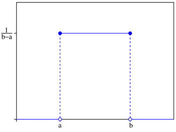 Figure 2.2.1: Uniform Distribution Probability Density Function
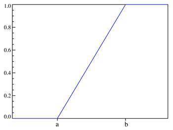 Figure 2.2.2: Uniform Distribution Cumulative Distribution
Function
Figure 2.2.2: Uniform Distribution Cumulative Distribution
Function a ~ The minimum repair time
b ~ The maximum repair time
Parameters required to model uniform distribution:
T ~(μ, σ)
The location parameter, μ = a
The scale parameter, σ = b - a
For a < t < b
Probability density function:
f(t) = 1 / σ
Cumulative distribution function:
F(t) = (t - μ) / σ
Inverse cumulative distribution function:
tp = μ + σp
Expected value:
E(T) = μ + σ / 2
For the example in Table 2 the element is out of service on average 9% of the year and outage events vary in duration from 6 to 36 hours with uniform probability.
| Property | Value | Units | Band |
|---|---|---|---|
| Forced Outage Rate | 9 | % | 1 |
| Min Time to Repair | 6 | hrs | 1 |
| Max Time to Repair | 36 | hrs | 1 |
2.3. Triangular Distribution
Repair time happens from a minimum to a maximum value with the mode value known.
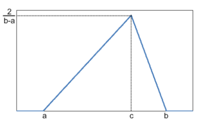 Figure 2.3.1: Triangular Distribution Probability Density
Function
Figure 2.3.1: Triangular Distribution Probability Density
Function 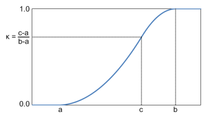 Figure 2.3.2: Triangular Distribution Cumulative Function
 a ~ The minimum repair time
b ~ The maximum repair time
c ~ The mode repair time
Parameters required to model triangular distribution:
tp = μ + σp
The location parameter, μ = a
The scale parameter, σ = b - a
The shape parameter, κ = (c - a) / (b
- a)
For a < t < b
Probability density function:
f(t) = 2(t-μ) / σ2κ for t ≤ c
f(t) = 2(μ+σ-t) / σ2(1-κ) for t ≥ c
Cumulative distribution function:
F(t) = (t - μ)2 / σ2κ for t ≤ c
F(t) = 1 - (μ+σ-t)2 / σ2(1-κ) for t ≥
c
Inverse cumulative distribution function:
tp = μ + σ√(κp) for p ≤ κ
tp = μ + σ(1-√[(1-κ)(1-p)]) for p ≥ κ
Expected value:
E(T) = μ + σ(1+κ) / 3
For the example in Table 3 the element is out of service on average 9% of the year and outage events vary in duration from 6 to 36 hours with 12 hours being the highest frequency.
| Property | Value | Units | Band |
|---|---|---|---|
| Forced Outage Rate | 9 | % | 1 |
| Min Time to Repair | 6 | hrs | 1 |
| Mean Time to Repair | 12 | hrs | 1 |
| Max Time to Repair | 36 | hrs | 1 |
2.4. Exponential Distribution
Repair times happen at a constant average rate, λ. That is, it does not matter how long the time since the last failure, the repair time will be the same. It is commonly used for high quality electronic circuits, or for components that exhibit wearout only after the expected technological life of the component.
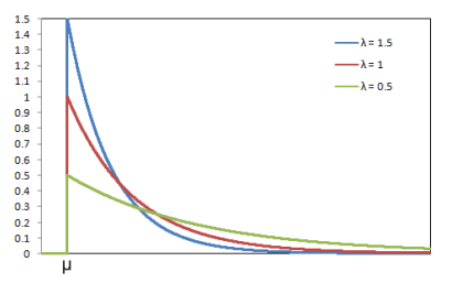 Figure 2.4.1: Exponential Distribution Probability Density
Function
Figure 2.4.1: Exponential Distribution Probability Density
Function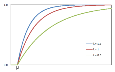 Figure 2.4.2: Exponential Distribution Cumulative Function
 a ~ The minimum repair time
λ ~ The rate parameter
Parameters required by PLEXOS to model exponential distribution:
T ~(μ, σ)
The location parameter, μ = a
The scale parameter, σ = 1 / λ
For t > μ
Probability density function:
f(t) = exp(-(t-μ)/σ) / σ
Cumulative distribution function:
F(t) = 1 - exp(-(t-μ)/σ)
Inverse cumulative distribution function:
tp = μ - σ.ln(1-p)
Expected value:
E(T) = μ + σ
In the following example the element is out of service on average 9% of the year and outage events with minimum duration of 6 hours and the rate of 1.
| Property | Value | Units | Band |
|---|---|---|---|
| Forced Outage Rate | 9 | % | 1 |
| Min Time to Repair | 6 | hrs | 1 |
| Repair Time Scalar | 1 | - | 1 |
2.5. Weibull Distribution
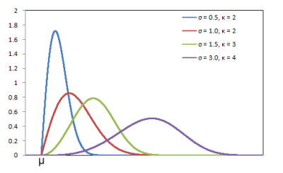 Figure 2.5.1: Weibull distribution probability density function
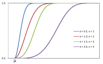 Figure 2.5.2: Weibull Distribution Cumulative Function
Parameters required to model Weibull distribution:
T ~(μ, σ, κ)
The minimum repair time, μ
The scale parameter, σ
The shape parameter, κ
Probability density function:
f(t) =
(κ/σ)[(t-μ)/σ]κ-1exp(-[(t-μ)/σ]κ)
Cumulative distribution function:
F(t) = 1 - exp(-[(t-μ)/σ]κ)
Inverse cumulative distribution function:
tp = μ + σ.(-ln(1-p))1/κ
Expected value:
E(T) = μ + σ.Γ(1+1/κ)
where gamma function, Γ(z) = ∫tz-1.e-tdt from 0 to ∞
ExampleIn the following example the element is out of service on average 9% of the year and outage events with minimum duration of 6 hours, the shape parameter of 2 and the scale parameter of 1.
| Property | Value | Units | Band |
|---|---|---|---|
| Forced Outage Rate | 9 | % | 1 |
| Min time to repair | 6 | % | 1 |
| Repair Time Shape | 2 | - | 1 |
| Repair Time Scale | 1 | - | 1 |
2.6. Lognormal
It is useful for modelling components with a decreasing repair time (due to a small proportion of defects in the population). It is used to describe time to failure for certain degradation processes.
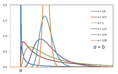 Figure 2.6.1: Lognormal distribution probability density function
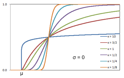 Figure 2.6.2: Lognormal distribution cumulative function
Parameters required by PLEXOS to model Lognormal distribution:
The minimum repair time, μ
The scale parameter, σ
The shape parameter, κ
For t > μ
Probability density function:
f(t) = (1/κ(t-μ)).φnor([ln(t-μ)-σ]/κ)
Cumulative distribution function:
F(t) = Φnor([ln(t-μ)-σ]/κ)
Inverse cumulative distribution function:
tp = μ + exp(σ+κ.Φnor-1(p))
Expected value:
E(T) = μ + exp(σ+κ2/2)
In the following example the element is out of service on average 9% of the year and outage events with minimum duration of 6 hours, the shape parameter of 2 and the scale parameter of 1.
| Property | Value | Units | Band |
|---|---|---|---|
| Forced Outage Rate | 9 | % | 1 |
| Min Time to Repair | 6 | hrs | 1 |
| Repair Time Shape | 2 | - | 1 |
| Repair Time Scale | 1 | - | 1 |
2.7. Smallest Extreme Value (SEV)
It can be used to model components with an increasing repair time.
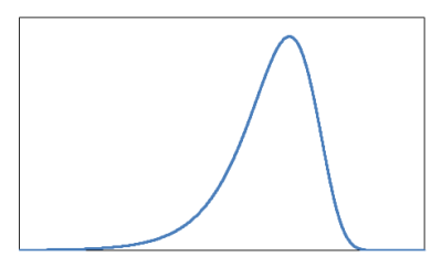 Figure 2.7.1: Smallest extreme value distribution probability
density function
Figure 2.7.1: Smallest extreme value distribution probability
density function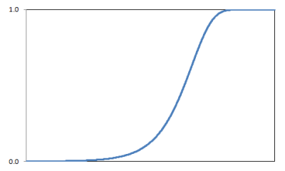 Figure 2.7.2: Smallest Extreme value distribution cumulative
function
Figure 2.7.2: Smallest Extreme value distribution cumulative
functionParameters required by PLEXOS to model SEV distribution:
T ~(μ, σ)
The location parameter, μ
The scale parameter, σ
For -∞ < t < ∞
Probability density function:
f(t) = (1/σ).exp((t-μ)/σ -
exp((t-μ)/σ))
Cumulative distribution function:
F(t) = 1 - exp(-exp((t-μ)/σ))
Inverse cumulative distribution function:
tp = μ + σ.ln(-ln(1-p))
Expected value:
E(T) = μ - 0.5772.σ
In the following example the element is out of service on average 9% of the year and outage events with the location parameter of 6 hours and the scale parameter of 1.
| Property | Value | Units | Band |
|---|---|---|---|
| Forced Outage Rate | 9 | % | 1 |
| Min Time to Repair | 6 | hrs | 1 |
| Repair Time Scale | 1 | - | 1 |
2.8. Largest Extreme Value (LEV)
It can be used to model components with an increasing repair time which remains constant after a period of time.
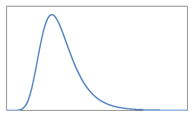 Figure 2.8.1: Largest extreme value distribution probability
density function
Figure 2.8.1: Largest extreme value distribution probability
density function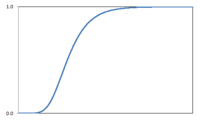 Figure 2.8.2: Extreme value distribution cumulative function>
Parameters required by PLEXOS to model LEV distribution:
T ~(μ, σ)
The location parameter, μ
The scale parameter, σ
For -∞ < t < ∞
Probability density function:
f(t) = (1/σ).exp(-(t-μ)/σ -
exp(-(t-μ)/σ))
Cumulative distribution function:
F(t) = exp(-exp(-(t-μ)/σ))
Inverse cumulative distribution function:
tp = μ - σ.ln(-ln(p))
Expected value:
E(T) = μ + 0.5772.σ
In the following example the element is out of service on average 9% of the year and outage events with the location parameter of 6 hours and the scale parameter of 1.
| Property | Value | Units | Band |
|---|---|---|---|
| Forced Outage Rate | 9 | % | 1 |
| Min Time to Repair | 6 | hrs | 1 |
| Repair Time Scale | 1 | - | 1 |
3. Planned (Maintenance) Outages
Generator, transmission line and gas pipeline planned outages can be input with the properties:
However, a complete forecast schedule of maintenance outages is
rarely available for all plant. The PASA simulation phase can
automatically schedule additional outages and time those outages and
time those outages appropriately at times of maximum reserve.
Further the maintenance class can be used to perform value-based
reliability analysis by optimally timing outages accounting for all
system costs and constraints.
4. Large-scale Resource Adequacy
Resource adequacy (RA) assessment aims to quantify loss of load expectation (LOLE) and/or loss of load probability (LOLP) within an energy system. This may involve generating hundreds if not thousands of outage and/or maintenance patterns for each Generator. On large scale power systems spanning thousands of generators, this can result in many large problems being solved (particularly with MT Schedule or ST Schedule). This can be computationally burdensome.
The computational burden can be efficiently reduced through the aggregation classes (Power Station and Battery Station). These classes aggregation individual assets together (i.e. to a geographical node), greatly reducing problem sizes. Outages and maintenances can still be generated for the aggregated units. This retains an effective representation of the problem for LOLE/LOLP quantification, which is the key aim of RA. Exact market reproduction including pricing forceast accuracy is of secondary concern.
5. References
[1] IEEE Std 762, "IEEE Standard Definitions for Use in Reporting Electric Generating Unit Reliability, Availability, and Productivity", 2008