Reliability Modelling With Monte Carlo Simulation
- Prerequisites
- Introduction
- Setup
- Formulation
- Required Sample Size
- Decomposition of Constraints and Storage
1. Prerequisites
Before reading this article, it would be useful to first read the article Planning and Random Outages.
2. Introduction
Configured correctly, PLEXOS is a powerful, fast and accurate Monte Carlo simulation engine highly suited to power system reliability analysis. This article provides a detailed guide to configuring the simulator for maximum performance when running in 'reliability mode' and some of the advanced features available to the analyst.
Monte Carlo reliability studies simulate the operation of the power system over a single or multi-year horizon across a wide range of scenarios. Central to these scenarios is modelling variations in the patterns of random, and planned, outages on Generator and/or Line and Gas Pipeline components. Other variations such as load or renewable energy sources (RES) are also useful.
These studies aim to forecast generation capacity reserves and reliability metrics, in particular, the Region Unserved Energy and Unserved Energy Hours. These results can then be compared to a standard i.e. acceptable level of unserved energy or hours of outage. For example, in the Australian NEM, the minimum standard is 0.002% unserved energy in any year.
3. Setup
3.1. Simulation Phases
The reliability run is generally set up with three-inter linked simulation phases:
- Preschedule/PASA: Generates patterns of random outages for 'unreliable' system elements (Generator, Line, and Gas Pipeline). The number of patterns is controlled by the Stochastic setting Outage Pattern Count, and optionally Reduced Outage Pattern Count.
- MT Schedule: Simulates across the entire horizon in long steps at a reduced level of temporal detail, allowing long term constraints and hydro releases to be optimized with sufficient 'look ahead'.
- ST Schedule: Solves the entire horizon in short steps (e.g. daily) with full temporal detail (half hour, 5-minute, 4-second for example). Information about long term constraints and hydro release policy is read from the solution to MT Schedule. Each outage pattern is run separately (Monte Carlo simulation).
Simulation phases are 'enabled' by adding the phase objects to the collections of the Model object. Every Model requires a Horizon object and this controls how the ST Schedule phase runs. An example is given in Figure 1. Here a two-year horizon is solved by ST Schedule in 730 one-day steps at half-hour resolution. This means that each simulated day will have 48 time periods and resources such as hydro will be optimized within each day. However, constraints and hydro storage longer than one-day will require 'decomposition' by MT Schedule so ST Schedule can deal with them. This decomposition is automatic when MT Schedule is enabled. The resolution of MT Schedule is controlled by the settings for the associated object rather than on the Horizon page.
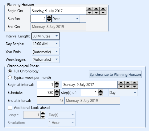 Figure 1: Example Horizon Setting
3.2. Simulation Settings
Example simulation settings for reliability are illustrated in the screenshots in Figures 2-7. Where settings are not shown in these figures, default values are assumed. Table 1 discusses these settings. The settings below are based on a specific study and are suggestions only. You should adapt your settings to suit your requirements and study system.
| Class | Setting | Notes |
|---|---|---|
| Horizon | Periods per Day = 48 | Set to reflect desired resolution of the ST Schedule simulation e.g. half-hourly resolution is 48 periods per day. |
| - | Chrono Step Type = "Day" | Steps of day duration allow hydro to be reoptimized within each 24-hour period. |
| PASA | N/A | This phase is not required. Forced outages are computed whether or not PASA is enabled. Only enable PASA if you want maintenance outages to be automatically scheduled. |
| MT Schedule | At a Time = 2 | This controls how long the MT Schedule step is. It may be desirable for MT Schedule to optimize the entire horizon (of two years for example) in one optimization. This avoids any artificial annual boundary at the end of MT Schedule steps. By default MT Schedule will simulate in annual steps. |
| - | LDC Type = "Day" | Matching the LDC type to the chronological step type gives the best decomposition results. |
| - | Blocks = 3 | The number of blocks (time periods) in each LDC can be tailored for best performance/accuracy of the hydro decomposition. |
| - | Heat Rate Detail = "Simplest" | Detailed heat rate modelling is generally not useful for reliability modelling. This setting will reduce the number of equations and complexity in the simulation and result in a faster runtime. |
| ST Schedule | Stochastic Method = "Independent samples (Parallel)" | This is the fastest execution mode for Monte Carlo simulation when the number of outage patterns is small. The memory use should be monitored however as the number of outage patterns increases, and with a large number of outage pattern it may be faster to run "Sequential". |
| - | Heat Rate Detail = "Simplest" | As above |
| Transmission | Internal VoLL = $14200 | This is the penalty applied to unserved energy ("energy not served") in the optimization problem. It should match the same penalty used in the market software. |
| - | Interruption Sharing | If this is enabled, causes shortages to be shared between interconnected regions in proportion to their demand rather than 'simply' minimizing the total shortage. This should be set consistent with the market rules of the system being studied. |
| Production | Dispatch by Power Station | By default Power Station objects are enabled if defined. This will speed up the simulation, but might cause issues with custom transmission constraints for example. |
| Stochastic | Outage Pattern Count = n | n is the number of required outage patterns in Monte Carlo simulation. |
| - | Reduced Outage Pattern Count = m | m is the number of outage patterns simulated (see below). |
| Diagnostic | Step Summary = "No" | This makes the steps run in "quiet" mode which is much faster for large Monte Carlo models. |
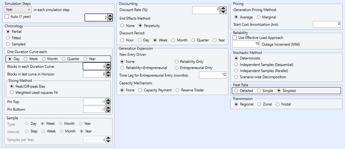 Figure 2: Example MT Schedule Settings
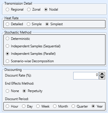 Figure 3: Example ST Schedule Settings
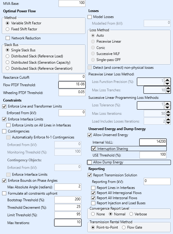 Figure 4: Example Transmission Settings
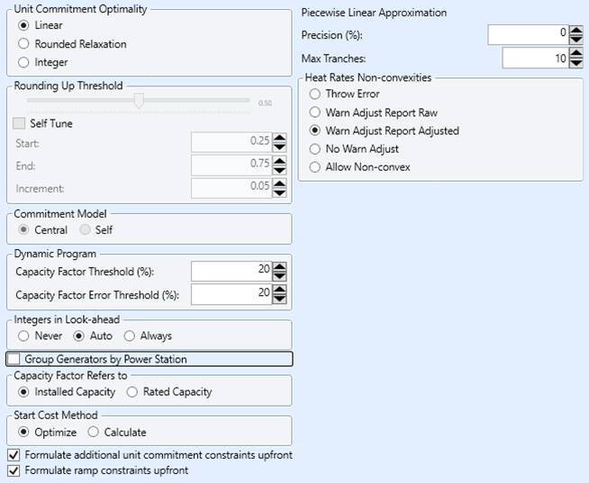 Figure 5: Example Production Settings
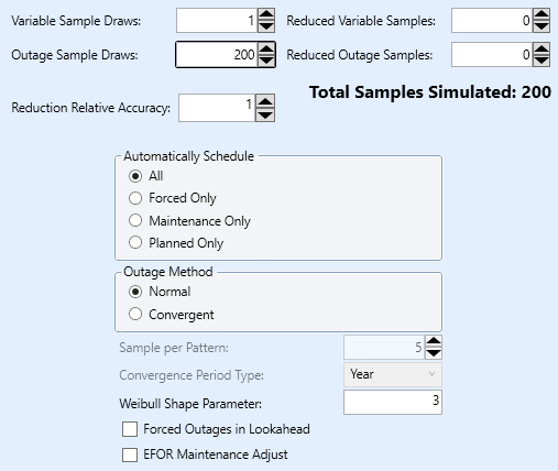 Figure 6: Example Stochastic Settings
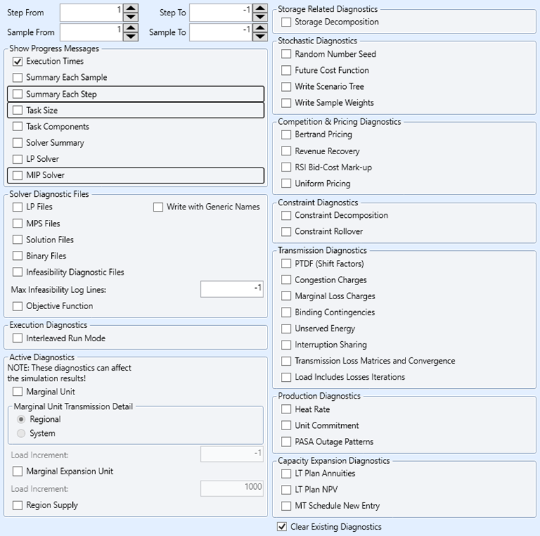 Figure 7: Example Diagnostic Settings
3.3. Report Selections
Report selections should be made sparingly to reduce runtime. Reliability runs are focused on capacity and thus most financial report values can be excluded. Figure 8 shows suggested report settings. Tick the 'Samples' box for each output that should be output for every outage pattern. Minimize the number of such properties to improve performance and reduce the size of the resulting solution database. Figure 9 shows a minimal set of report selections being Unserved Energy and Unserved Energy Hours.
If you require other outputs try to minimize the number of outputs that are reported 'by sample' and/or with statistics i.e. some outputs might only be required as averages across all samples.
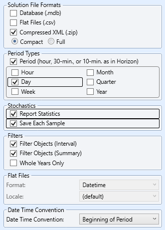 Figure 8: Example Report Settings
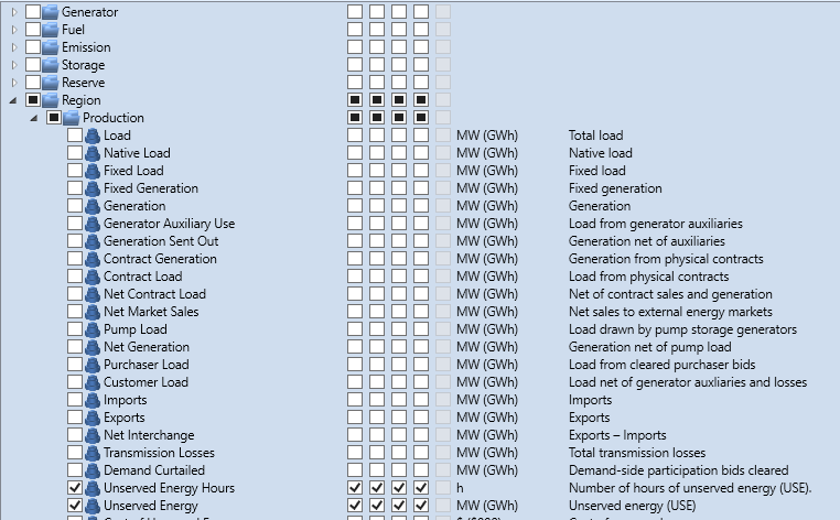 Figure 9: Minimal Report Selections
4. Formulation
To maximize performance it is important to reduce the complexity of the input used, which translates directly to the size and complexity of the optimization problems formulated and solved by the simulator. You can use Scenario objects to remove detail from the simulation, so it is not necessary to develop a special version of your database for reliability, just careful use of scenarios will do.
4.1. Basic and Optional Inputs
A minimum set of inputs could be like those in Table 2.
Table 2: Minimum set of inputs for reliability studies
| Class | Property | Description |
|---|---|---|
| Region | Load | The load that the generation system must meet. |
| Line | Max Flow | Maximum import or export on a transmission line. |
| Generator | Units | Number of units of Max Capacity in size |
| - | Max Capacity | Generation capacity of each unit |
| - | Rating | Rating of each unit. This is useful to define a dynamic limit on the production from renewable generation sources, or a summer/winter rating for conventional plant. |
| - | Forced Outage Rate | Average unavailability due to random outage. Refer to forced Outage rte Denominator for interpretation of this property. |
| Line | Forced Outage Rate | Forced outage rate for transmission. |
Other inputs that are relevant to reliability are in Table 3. Note that this is not an exhaustive list.
Table 3: Other inputs relevant to reliability studies
| Class | Property | Description |
|---|---|---|
| Region | DSP Bid Quantity | Demand-side participation which can be defined in multiple price bands |
| - | DSP Bid Price | - |
| - | VoLL | The maximum price when unserved energy occurs. |
| Generator | Min Stable Level | The minimum operating level of generating unit when 'on' and past its run-up period. |
| - | Outage Rating | Defines a partial outage state. This is used in bands with forced outage rate to define multiple states. |
| - | Max Ramp Up | Maximum ramping rates for a generating unit between minimum stable level and maximum capacity. |
| - | Max Ramp Down | - |
| Line | Outage Max Rating | Defines a partial outage state. |
4.2. The Objective Function
In the simplest case, the objective function of the simulation need only include penalty costs on unserved energy (and demand-side participation if that is relevant). Other 'production costs' are not relevant to the problem of minimizing unserved energy. However, in many instances, this ideal case is not valid, for instance:
- where hydro-thermal coordination requires a trade-off between the present value of hydro releases and future thermal cost, the cost of shortage alone is probably insufficient.
- where the unit commitment and/or dispatch need to be realistic for modelling transmission constraints or system stability, or when modelling the effect of unit start up and ramp constraints.
Thus, at least a basic 'merit order' of generation is generally necessary. Unless fuel supply is a likely cause of generation shortage, there is no need to model fuels in the simulation. To keep your Fuel objects in the database, but exclude them from the reliability simulation set the Generator Fuels Is Available to zero. Table 4 lists the basic cost parameters for thermal plant. No costs are required for RES such as wind, solar, hydro, etc.
Table 4: Basic thermal cost data
| Class | Property | Description |
|---|---|---|
| Generator | Fuel Price | Price of fuel to the generator |
| - | Heat Rate | Fuel used per unit of electric production |
| - | VO&M Charge | Variable operations and maintenance charge per unit of electric production |
4.3. Intermittent Generation
In 'normal' simulation mode, intermittent generation, such as RES, is handled by Variable objects applied to capacity properties such as Rating, Rating Factor, Fixed Load or Natural Inflow. These are then sampled according to the Stochastic setting Risk Sample Count.
This approach can work in reliability mode too i.e. you can specify running multiple outage patterns and multiple variable samples in one simulation.
An alternative, using partial outage states, which keeps intermittent generation inside the outage pattern framework is described in the Intermittent Generation section of the LOLP article.
4.4. Storage
Storage such as hydro and battery energy storage can and should be modelled in full detail in reliability studies.
4.5. Gas
Where gas delivery is potential source of shortage in electrical production the gas system can and should be modelled in full detail.
4.6. Reserves
Commonly, many ancillary services such as spin up/down, regulation and the like, modelled as reserve objects, can be excluded from reliability studies, In a shortage situation, these provisions are often relaxed, and in that case, continuing to enforce them during a shortage is 'double counting'.
4.7. Constraints
Custom constraints implemented as Constraint objects that can be included in the reliability run. These might include transmission constraints more complex than a simple line or interface limit, or additional technical constraints on the generation system.
The most important consideration here is the setting of Penalty Price. If the constraint is unbreakable, then the default will enforce the constraint 'at all cost', but for constraints that can be relaxed in times of potential shortage, it is important to consider the interaction between Penalty Price and the Internal VoLL, and also the implied 'ranking' of constraints based on their penalty prices.
5. Required Sample Size
Sufficient samples must be run to guarantee convergence of the unserved energy estimate. By "sample" we mean the setting Stochastic Outage Pattern Count i.e. the number outage 'draws' or 'patterns' simulated.
How many samples are enough?
5.1. Convergence and Repair Time
It is well known that convergence of unserved energy is affected by the duration of outages. For example, a 1000 sample run with 'default' repair times of 24 hours might produce a convergence chart like Figure 10. The standard error of estimate for the mean here is 0.0064. The same set of simulations but with a repair time of 30-minutes converges as in Figure 11. The same standard error of estimate is achieved with 40 samples and the estimate at 1000 samples has 95% confidence with ±8%.
The caveat is that the distribution of outage severity is also affected by the repair time. Thus, if the outage severity distribution is of interest, the 'accurate' repair times should be used and a commensurably larger sample size. This is illustrated in Figure 12 and Figure 13 which show the outage severity distributions for repair time of 24 hours and half-hour respectively.
In conclusion, a large sample size is required, but careful consideration needs to be given to the input parameters for repair time. Research suggests that sample sizes in the 500-2000 range are generally sufficient for convergence to a reasonable standard error.
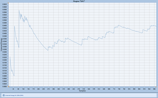 Figure 10: Unserved Energy Estimate Convergence MTTR = 24 hours
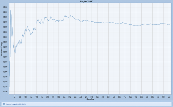 Figure 11: Unserved Energy Estimate Convergence MTTR = 0.5 hours
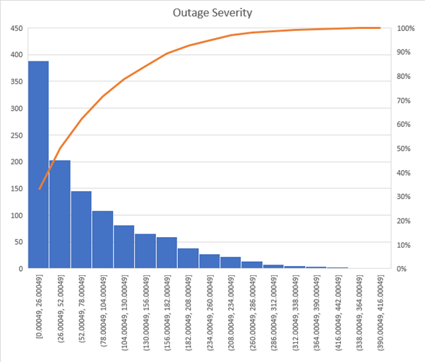 Figure 12: Outage severity MTTR=24 hours
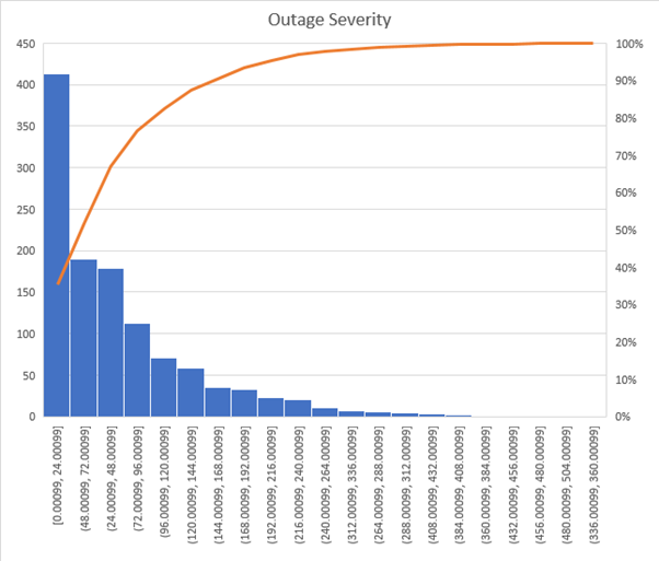 Figure 13: Outage Severity MTTR=half hour
5.2. Outage Pattern Sample Reduction
Outage patterns are similar in concept to samples of stochastic variables like hydro inflows or wind speed. The latter variables are modelled using Variable objects and the number of samples of these variables drawn in a simulation is controlled by the Stochastic setting Risk Sample Count. The simulator can draw a large pool of samples but reduce them automatically to a concise set for simulation. This is controlled by the Stochastic setting Reduced Sample Count. Refer to that topic for details of how the reduction is performed.
In the same manner, the outage patterns can be reduced to a concise set for simulation. Figure 14 illustrates how to set up the Stochastic settings to generate a pool of 1000 outage draws/patterns and have them automatically reduced to 50 for simulation. Figure 15 illustrates how the unserved energy estimate converges across the original 1000 samples but based on the 50 simulated samples. The 50 simulated samples are selected from the original population of 1000 using statistical methods and this means the confidence intervals are tighter than if we had simply simulated the first 50 samples or a random set of 50 samples.
Thus, it is possible to converge on an acceptable standard error of the unserved energy estimates from a reduced set of outage patterns. In the illustrated case the runtime is improved better than 20 times compared to simulating all the outage patterns.
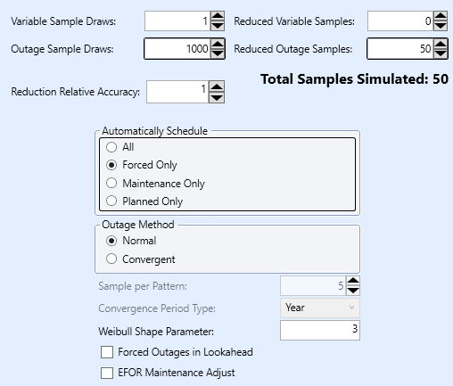 Figure 14: Stochastic settings for outage pattern sample reduction
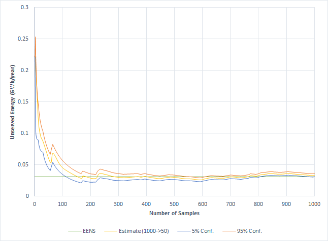 Figure 15: Convergence of Unserved Energy Estimate (1000->50)
6. Decomposition of Constraints and Storage
For an introduction to constraint decomposition, please refer to the article Constraint Decomposition. Broadly speaking, MT Schedule will decompose (break into smaller pieces) constraints that ST Schedule cannot resolve in its step including look-ahead.
Decomposition of constraints and storage presents unique challenges in the context of reliability modelling. Constraints such as Generator Max Energy and the trajectory for Storage End Volume will affect the capacity available for generation production at times of potential shortage. Should the decomposition i.e. allocation of the constraints and storage releases, be imperfect, then production resources might not be available at the 'right' time and as a result Region Unserved Energy could be overstated.
Concretely, this problem only occurs when decomposition is actually required. If all constraints are short enough that the step length of ST Schedule can handle them, then there is no issue. For example, if the longest such constraint is weekly and ST Schedule runs in weekly steps (or daily with look-ahead enough for a week), it can handle all the constraints optimally. However, even if weekly constraints are the longest, you might prefer, for performance reasons, to run ST Schedule in daily or shorter steps, or your constraints might be monthly or annual, and this is where MT Schedule decomposition comes in.
For example, consider the case of weekly energy constraints being decomposed so that ST Schedule can run in daily sized steps. Let's assume MT Schedule runs with MT Schedule Transmission Detail = "Regional" but ST Schedule Transmission Detail = "Nodal" or your have custom constraints that only apply to ST Schedule. Clearly, the solution from MT Schedule will be unaware of some constraints that could impact the delivery of generation via the transmission network and thus the decomposition of energy and/or storage might be too 'optimistic'.
How do we resolve this?
There are two possible solutions:
- Run ST Schedule with sufficient look-ahead to cover any constraint and Storage to 'see' far enough ahead to avoid a shortage. An example is shown in Figure 16. Each step is one day long but has six further days of look-ahead. This look-ahead period is run at a lower resolution so as not to consumed too much additional time, while still providing the benefits of looking ahead.
- Rely on ST Schedule to automatically 'borrow' energy from the future at a penalty cost.
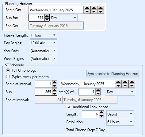 Figure 16: Horizon settings with look-ahead
The 'borrow' method is automatic for Storage and allows variations from the storage trajectory determined by MT Schedule at a penalty price related to the shadow price of storage from that simulation phase. The details of this penalty function are available via the Diagnostic Storage Decomposition.
For Constraint objects, both user-defined and those implied by properties like Generator Max Energy borrowing from future periods is automatic at a penalty of Transmission Internal VoLL. This only applies however to energy constraints and not to fuel or other constraints.
This 'borrow' process can be monitored via the Diagnostic Constraint Rollover. 'Rollover" refers to how constraints are tracked as the simulation 'rolls' through steps and constraint activity 'carry' and 'borrow'. Borrowing can also be seen in the Constraint Slack reporting as a negative number as in the following example:
| Datetime | Activity | Slack | Violation | Hours Binding (h) | RHS | Price ($) |
|---|---|---|---|---|---|---|
| 1/01/2002 | 0.01 | -0.005 | 0 | 24 | 0.005 | 14999.99 |
| 2/01/2002 | 0.155 | 0.005 | 0 | 24 | 0.16 | 23.33 |
| 3/01/2002 | 0.16 | 0 | 0 | 24 | 0.16 | 23.33 |
| 4/01/2002 | 0.16 | 0 | 0 | 24 | 0.16 | 23.33 |
| 5/01/2002 | 0.19 | 0 | 0 | 24 | 0.19 | 13.33 |
| 6/01/2002 | 0.16 | 0 | 0 | 24 | 0.16 | 23.33 |
| 7/01/2002 | 0.165 | 0 | 0 | 24 | 0.165 | 23.33 |
| 8/01/2002 | 0.14285714286 | 0 | 0 | 24 | 0.14285714286 | 23.33 |
Here the constraint 'borrows' in the first day in order to avoid unserved energy and pays it back in the next step.
See also: