Transmission - Security Constrained Unit Commitment and Dispatch
Contents
- Introduction
- Calculation of Contingency Shift Factors
- Generator Contingencies
- N-x Contingency Analysis
- SCUC and Interfaces
- SCUC and Interfaces
- Example
1. Introduction
Security constrained unit commitment (SCUC) finds the optimal unit commitment and dispatch solution subject to the transmission being feasible if any defined contingency (such as the loss of a line or generator) should occur. The SCUC algorithm in PLEXOS computes contingency shift factors (also called generation-shift sensitivity factors) which define how much of the flow lost during a contingency will appear on other lines in the network: these factors are used to monitor and enforce the contingency constraints. The resulting dispatch is more conservative and at higher cost, but reflects more accurately the actual system operation. The following discussion is adapted from (A.J. Wood, 1996).
2. Calculation
First we show how to derive the generation-shift sensitivity factors. We start with the standard power flow equation for the linearized DC-OPF presented above:
θ = [X]P
Since the DC-OPF is a linear model, we may calculate perturbations about any given set of system conditions by using the same model. Thus, if we are interested in the changes in bus phase angels, Δθ for a given set of changes in the bus power injections, δP, we can use the following calculation.
Δθ = [X]ΔP
It is assumed that the power on the slack bus(es) is equal to the sum of the injections of all the other buses. Similarly, the net perturbation of the slack bus(es) (in the equation above) is the sum of the perturbations on all the other buses.
Suppose that we are interested in calculating the generation shift sensitivity factors for the generator on bus i. To do this, we will set the perturbation on bus i to +1 and the perturbation on all other buses to zero. We can then solve for the change in bus phase angles using the matrix calculation in the following equation.
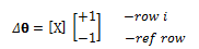
The vector of bus power injection perturbations in the above equation represents the situations when a 1 p.u. power increase is made at bus i and is compensated by a 1 p.u. decrease in power at the slack bus. The Δ"θ" values are thus equal to the derivative of the bus angles with respect to a change in power injection at bus i. Then, the required sensitivity factors are:
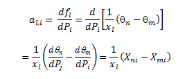
where:
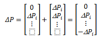
A line outage may be modelled by adding two power injections to a system, one at each end of the line to be dropped. The line is actually left in the system and the effects of it being dropped are modelled by injections. Suppose line k from bus n to bus m were opened by circuit breakers. Note that when the circuit breakers are opened, no current flows through them and the line is completely isolated for the remainder of the network. To model this situation the breakers can remain closed but injections δPn and δPm can be added to bus n and bus m, respectively counteracting the original flow on the line.
If δPn = δP̃nm , where δP̃nm is equal to the power flowing over the line, and δPm = -δP̃nm we will still have no current flowing through the circuit breakers even though they are closed. As far as the remainder of the network is concerned, the line is disconnected.
Using the equation relating to δθ and δP , we have:
Δθ = [X]ΔP
where:
define:
θn , θm , Pnm to exist before the outage, where P_nm is the flow on line k from bus n to bus m
δθn , δθm , δPnm to be incremental changes resulting from the outage
\[\tilde{\theta}_{n}\] , \[\tilde{\theta}_{m}\] , \[\tilde{P}_{nm}\] to exist after the outage
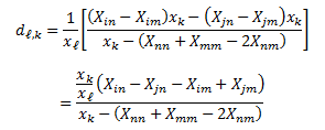
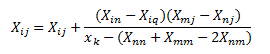
The outage modelling criteria requires that the incremental injections δPn and δPm equal the power flowing over the outaged line after the injections are imposed. Then if we let the line reactance be xk:
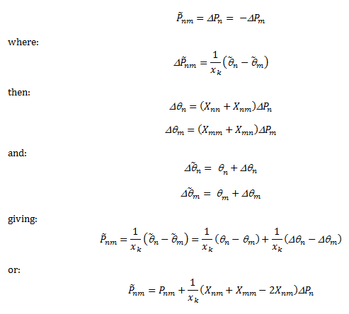
Then (using the fact that P̃nm is set to δPn):
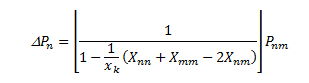
Define a sensitivity factor δ as the ratio of the change in phase angle θ, anywhere in the system, to the original power Pnm flowing over the line nm before it was dropped. This is:
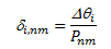
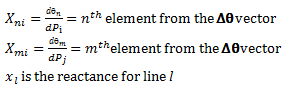
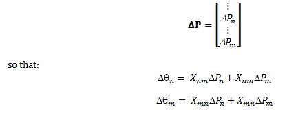
If neither n nor m is the system references bus, two injections, δPn and δPm, are imposed at buses n and m respectively. This gives a change in phase angle at bus i equal to:
δ θi = Xin Pn + Xim δPm
Then using the relationship between δPn and δPm, the resulting δ factor is:
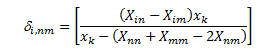
If either n or m is the reference bus, only one injection is made. The resulting factors are:
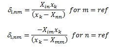
If bus i itself is the reference bus, then δi,nm=0 since the reference bus angle is constant. The expression for dl,k is:
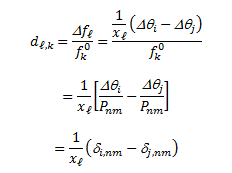
If neither i nor j is the reference bus:
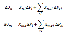
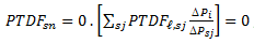
3. Generator Contingencies
Generation Shift Factor Calculations for the Single Slack
The PTDF is calculated as follows:
δθ=[X]δP
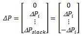
Where line l connects from bus n to bus m. Let the power injection change at bus i be one MW, δPi, and the slack bus will absorb same amount of power, δPslack=-δPi.
The power angle changes at bus n and bus m are
δ θn = Xn,i δPi
δ θm = Xm,i δPi
Then, the flow change at line l is
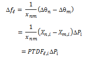
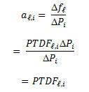
Then the generator shift factor from bus i to line l is
Generation Shift Factor Calculation for the Distributed Slack
In the distributed slack case, one MW injection at bus i will be absorbed by multiple slack buses.
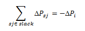
where bus sj is one of the slack buses. In the form of vector, the bus injection at bus i and the slack buses is:
Then power angle changes at bus n and bus m are
The flow change at line l is:
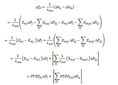
Then the generator shift factor from bus i to line l is
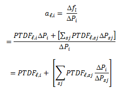
From this equation, we notice that there is an extra term,
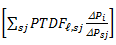 , in the generator shift factor for the distributed slack as opposed to the single slack bus. In the single slack bus case, δPsj=0 and δPsn=-δPi , and also θsn=0 which results in
 and αl,i is reduced to PTDFl,i as shown above.
Flow Constraint Changes due to the Generator Outage
In both cases of single or distributed slack, the flow constraint for the generator outage bus i is:
flmin ≤ fl0 - αl,i δ Pi = fl0 - αl,i Pi0 ≤ fimaxWhere Pi0 is the pre-contingency generation from the generator at bus i.
4. N-x Contingency Analysis
The SCUC in PLEXOS can also support the "N-x" contingency analysis, a standard of North American Electric Reliability Corporation (NERC) that ensures "two or more simultaneous contingencies will not propagate into a cascading blackout".
Three kinds of transmission elements can be selected as contingency object, Line, Transformer and Generator. Multiple elements selected in one contingency object will automatically enable the N-x contingency analysis in PLEXOS.
There are two important principles for DC-OPF based N-x contingency analysis:
- All the contingency elements are coupled together. The post-contingency solution for N-x is not equal to the sum of all the N-1 conditions.
- The calculation sequence of the contingency elements will not affect the final post-contingency power flow solution.
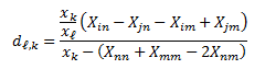
The contingency shift factor derived in section 9.1 is still applicable as below.
However, the [X] matrix of the network has to be updated every time after an AC line or AC transformer outage. The impedance matrix, [X] matrix is updated by eliminating the susceptance contributions from the outaged element, i.e. line k (from n to m).
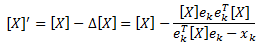
where ek is the line k connection vector,
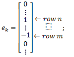
xk is the susceptance of line k.
Each element of [X] is updated as below:
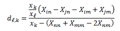
Example
If an N-2 contingency is defined as {k, w}, where AC line k and w are set as contingency objects. The post-contingency power flow after line k (from n to m) outage on line l will be calculated as
fl' = fl0 - dl,k fk0where fl0 and fk0 are the pre-contingency power flows;
dl,k is the contingency shift factor calculated based on original network.
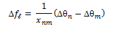
In order to further analysis the line w (from a to b) outage, the network topology and susceptance matrix have to be updated by taking line k out. The new [X] matrix is then expressed as [X]-k.
Then the post-contingency power flow on line l will be finally calculated as
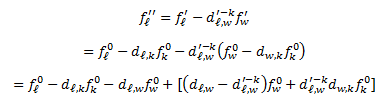
where -> fl0, fk0 and fw0 are the pre-contingency power flows;
f'l and f'w are the power flows after line k outage;
dl,k and dl,w are the contingency shift factor calculated based on original network;
dl,w'-k is the contingency shift factor calculated based on the network after line k outage.
The generator outage in N-x contingency analysis is generally the same as in N-1 cases.
5. SCUC on Large-scale Networks
SCUC is a challenging problem to solve because the number of constraints implied is very large. For each contingency we are considering the limits on all lines by computing their post-contingency flow. Thus the number of flow limits imposed can be huge. To limit the number of limits considered in SCUC do the following:
- Set the Transmission SCUC Constraint Voltage Threshold attribute to set a voltage level at or above which line limits are monitored; and/or
- Limit the set of Line limits considered by adding specific Line objects into the Contingency Monitored Lines collection for each Contingency
Using the latter method it is possible to consider a large number of contingencies even on a large-scale network.
6. SCUC and Interfaces
Interface objects are normally defined with limits (Max Flow and Min Flow) that account for contingencies, thus the PLEXOS SCUC algorithm does not monitor post-contingency flows on Interface flows by default. You can however select Interface objects whose post-contingency flows should be monitored using the Contingency Monitored Interfaces collection i.e. for each Contingency add the set of Interface objects to be monitored into the collection.
7. Example
We illustrate the use of SCUC in PLEXOS using the 7-Node network described in Section 9.6. We solve three cases:
- Economic dispatch and optimal power flow ignoring contingencies and losses which is shown in Figure 1.
- Case 1 with a contingency defined on a single line.
- Case 1 but with all lines as contingencies.
In all cases PLEXOS will compute the shift factors for the network based on single slack bus, however distributed slack would work similarly. The shift factors are shown in Table 17.
Contingency on single line
In this case we define a contingency on Line "2_5". This is done in PLEXOS by creating a Contingency object and placing the Line "2_5" in the Contingency Lines collection for that Contingency. The Contingency Is Enabled property is then set to "Yes". Finally the SCUC must be enabled in Transmission settings (see the "Security Constrained Unit Commitment (SCUC)" switch in Figure 6).
When this case is run in PLEXOS the contingency shift factors are computed for the case of Line "2_5" going out of service. These factors are shown in Table 7. For example, for the loss of one megawatt of flow from Node "2" to Node "5" the flow between Node "2" to Node "3" will increase by 0.1485.
Table 7: Contingency Shift Factors
| Node From | Node To | Contingency |
|---|---|---|
| 1 | 2 | -0.09217 |
| 1 | 3 | 0.09217 |
| 2 | 3 | 0.1485 |
| 2 | 4 | 0.18861 |
| 2 | 5 | 0 |
| 2 | 6 | 0.57073 |
| 3 | 4 | 0.24067 |
| 4 | 5 | 0.42927 |
| 5 | 7 | -0.57073 |
| 6 | 7 | 0.57073 |
The results for this case are illustrated in Figure 4. Compared to Figure 1 the total system cost has increased from 15113.45 to 15603.43. The generation pattern changes so that when if the flow on Line "2_5" is lost the post-contingency flows on the other lines will not exceed their thermal ratings. In the solution file PLEXOS reports the Contingency Shadow Price of 21.02. Thus, although no line is congested 'pre-contingency' there are still separations in nodal prices as in Table 8.
Table 8: Nodal pricing with single contingency
| Node | Price ($/MWh) | Energy Charge ($/MWh) | Congestion Charge ($/MWh) |
|---|---|---|---|
| 1 | 14.6 | 14.6 | 0 |
| 2 | 15 | 14.6 | -0.4 |
| 3 | 12.66 | 14.6 | 1.94 |
| 4 | 12.03 | 14.6 | -9.43 |
| 5 | 24.02 | 14.6 | -9.43 |
| 6 | 17.26 | 14.6 | -2.66 |
| 7 | 21.77 | 14.6 | -7.17 |
 Figure 4: 7-node with single line contingency
Contingencies on all Lines
We define contingencies on all lines by creating one Contingency object for each Line and adding that line to the contingency. The solution for this case is illustrated in Figure 5. The contingency shadow prices are shown in Table 9 and nodal prices in Table 10.
 Figure 5: 7-node with contingencies on all lines
Table 9: Contingency Shadow Prices
| Contingency | Is Binding (Yes/No) | Shadow Price ($/MW) |
|---|---|---|
| 1_2 | 0 | 0 |
| 1_3 | 0 | 0 |
| 2_3 | 0 | 0 |
| 2_4 | 0 | 0 |
| 2_5 | -1 | 9.95 |
| 2_6 | -1 | 1.57 |
| 3_4 | 0 | 0 |
| 4_5 | 0 | 0 |
| 5_7 | 0 | 0 |
| 6_7_1 | -1 | 5.03 |
| 6_7_2 | 0 | 0 |
Table 10: Nodal pricing with all lines as contingencies
| Node | Price ($/MWh) | Energy Charge ($/MWh) | Congestion Charge ($/MWh) |
|---|---|---|---|
| 1 | 14.95 | 14.95 | 0 |
| 2 | 15 | 14.95 | -0.05 |
| 3 | 14.69 | 14.95 | 0.26 |
| 4 | 14.6 | 14.95 | 0.35 |
| 5 | 23.34 | 14.95 | -8.39 |
| 6 | 17.71 | 14.95 | -2.76 |
| 7 | 21.77 | 14.95 | -6.82 |