Transmission - Loss Modelling
Contents
- Introduction
- Definitions
- Loss Data
- Loss Models
- Loss Models in FS-OPF
- Loss Models in VS-OPF
- Losses Embedded in the Load
- Special Loss Functions
- Approximating Losses Using a Penalty Function
1. Introduction
This section describes the formulation and solution algorithms available in PLEXOS for modelling power system losses.
2. Definitions
We use the following definitions:
Loss
Line thermal losses are a quadratic function of flow. For flow on path j we have:
Lj= rj fj2 where rj is the resistance (p.u.) on the path, and fj is the power flow on the path.
Thus the total system losses are the sum of these path flows:
Note that in the VS-OPF, line flows and losses are modelled directly in the formulation, but in the FS-OPF the line flows are implied by the vector of bus injections and the shift factors. In the FS-OPF we use another matrix of factors called the B-matrix to determine the total system losses for any given set of node injections.
B-matrix
The B-matrix defines the system losses thus:
L = PT BP
where:
- L is the total losses in the AC system
- P is the vector of power injections at the nodes in the network
The elements of B are calculated from the shift-factor matrix (D) and the vector of path resistances R thus:
where:
path j flows from bus k to bus l.
Marginal Loss
The associated marginal loss is the first-order derivative of the loss function w.r.t. the real power flow:
δj = 2rjfj
Marginal Loss Factor
In the context of modelling a power system:
- Losses are loads in the power system i.e. the total generation in the system is equal to the customer load plus transmission losses.
- Marginal losses generate differentials in nodal prices i.e. when power is flowing (unconstrained) from bus k to bus l along path j: λl=(1+δj ) λk and likewise when power is flowing from l to k: λk=λl / (1+δj).
- The ratio of prices λl / λk implied by marginal losses is called the marginal loss factor between node l and node k
3. Loss Data
In PLEXOS, losses can be associated with lines and transformers. For lines there are a number of ways to define the loss function, but for transformers you must use the Resistance property. Lines provide more options because they can be used to represent collections of lines in a notional interconnector, or DC lines, either of which could have more complex loss functions than just quadratic. For details on loss functions defined other than with resistance see the Section 8.7. Line or transformer resistances are entered per unit (p.u.) with the MVA base set using the Transmission MVA Base setting. Resistance can be defined on both AC and DC lines.
4. Loss Models
Adding modelling of losses to the simulation of a power system is a challenging exercise. The lossless DC-OPF is a linear model and is thus solved very efficiently using standard linear programming (LP) codes. Further, it is highly adaptable to the mixed-integer programming (MIP) environment which can take into account generator unit commitment constraints as well as other on/off decisions.
However, when we model losses, we are introducing non-linear (quadratic) equations to the mathematical problem. There are essentially three ways to adapt the existing solution method to handle this:
- Formulate the quadratic elements of the problem using non-linear programming. For the FS-OPF a quadratic representation of the B-matrix is formulated, and for the VS-OPF the line-by-line quadratic loss functions are formulated. This is the most accurate model.
- Approximate the quadratic function(s) with piecewise linear function(s) so the problem remains entirely linear and can be solved in an integrated manner using LP or MIP.
- Apply Successive Linear Programming (SLP) to the loss function(s), iterating on the Marginal Loss Factor at each injection point until convergence is reached.
- Calculate Generator Penalty Factors (GPF) and Generator Delivery Factors (GDF) to allocate marginal loss charges to injections. Then the approximated loss will be calculated by one-pass re-optimization.
PLEXOS provides options for modelling losses using all four approaches. The loss model is selected via the Transmission Loss Method setting. Combined with the two OPF algorithms (FS-OPF and VS-OPF) there are the set of combinations as follows:
Table 3: OPF and Loss Methods
| OPF Method | FS-OPF | VS-OPF |
|---|---|---|
| Loss Method | - | - |
| Quadratic | Yes | Yes |
| Piecewise Linear | Yes (default) | Yes (default) |
| SLP (Marginal Loss Factors) | Yes | No |
| Single-Pass GPF | Yes | No |
See Figure 6 for the Transmission settings that control these options. The loss method is set by the Transmission Loss Method attribute. Both OPF methods default to loss method "Piecewise Linear". This is chosen because it is the loss method most commonly associated with market-clearing engines that use DC-OPF e.g. New Zealand, Australia, Singapore, Ireland. Note that for the FS-OPF the SLP on Marginal Loss Factors is the fastest-executing method for large systems. This document describes these loss modelling algorithms in detail, and in what circumstances you would chose each model. NOTE: The selection of loss model affects loss modelling for AC lines only. Losses on DC lines are always modelled using the piecewise linear loss model.
5. Loss Models in FS-OPF
Quadratic
PLEXOS formulates the loss functions using conic optimisation. Conic problems are a special class of general quadratically-constrained (Qc) problems and have the desirable trait that they can be solved using the interior point method in the same way that linear (LP) and quadratic (Qo) problem can. Thus both a primal and a dual solution are available and algorithm solution time is predictable. The commercial solvers used by PLEXOS all provide support for either conic or Qc problems.
Thus the idea of the conic loss model is to take the direct approach of formulating the loss equation(s) as quadratic constraints. This has the advantage that the solutions are highly accurate w.r.t. both primal (losses) and dual (marginal loss factors and bus LMP). Not all solvers however support integer optimization combined with conic or Qo, therefore integer optimal unit commitment might not be available*.
In the PLEXOS implementation the FS-OPF solves the B-matrix loss formula (which defines total system losses) directly. This approach can lead to a large optimisation problem that is difficult to solve, thus either of SLP approaches usually solves faster and produces an equally accurate result with the tolerances defined.
* At the time of writing only the MOSEK solver supported solving integer problems with quadratic constraints.
Piecewise Linear
The Piecewise Linear method (which is the default method for FS-OPF) is essentially a replacement for the Quadratic method in the case where:
- Integer programming is required e.g. for unit commitment; and
- The solver being used does not support integer optimisation combined with quadratic constraints (QcQp).
This method solves the B-matrix via Separable Programming to approximate the losses in the AC network. The number of segments used in the approximation is controlled by the Transmission Max Loss Tranches setting. This should generally be set to a high number e.g. 20 or more to ensure accuracy.
SLP on Marginal Loss Factors
In this method rather than iterating on the terms of a Taylor Expansion of the B-matrix, PLEXOS iterates on the set of marginal loss factors for each injection node combined with a constant loss term. Thus the system energy-balance equation becomes:
where:
- MLFk is the marginal loss factor at node k
- c is the constant term of the loss approximation associated with the current MLF set
This formulation here is linear and is solved using SLP.
For the 7-Node example, the lossless solution is shown in Figure 1.Turning on losses with this loss method produces these messages
--------------------------------------------------------------------------------------------------------------------------------
 Iter                                           Real Loss (MWh)    Modeled Loss (MWh)    Absolute Gap (MWh)      Relative Gap (%)
 --------------------------------------------------------------------------------------------------------------------------------
 0                                                4.206716e+000        -3.552714e-013         4.206716e+000         1.000000e+002
 1                                                4.207822e+000         4.207737e+000         8.488731e-005         2.017370e-003
 2                                                4.207822e+000         4.207822e+000         0.000000e+000         0.000000e+000
 Loss method completed.  Exit status: TOLERANCE.  Iterations: 2.  Relative Gap: 0.000000e+000. Time: 0:00:00.033
 --------------------------------------------------------------------------------------------------------------------------------
In this case the loss convergence occurs in two iterations and the gap between the modelled and real losses is zero. The tolerance for convergence is controlled by the Transmission Loss Tolerance setting. An iteration limit can be set via the Transmission Max Loss Iterations setting. In general this method converges quickly and is relatively fast and efficient compared to the other approaches. The solution including losses for the 7-Node case is shown in Figure 2.
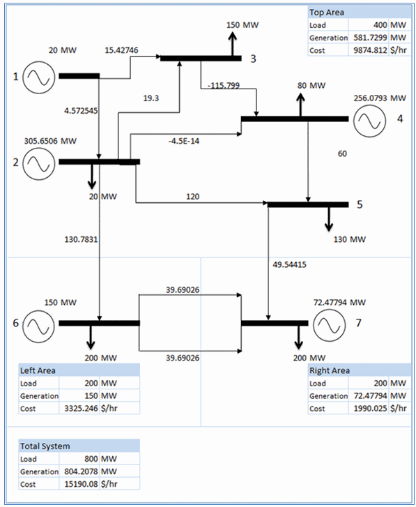 Figure 2: Dispatch Including Losses
Note that when integer optimisation is required e.g. for unit commitment when Production Unit Commitment Optimality is set to "Integer Optimal" or "Rounded Relaxation", PLEXOS must iterate between the convergence of losses and the unit commitment to find a reasonable solution.
Single-Pass GPF
It is an approximation loss method, applying to nodal model detail. The effects of marginal losses are reflected through the use of penalty factors and delivery factors.
Reference: Fangxing Li, Jiuping Pan and Henry Chao, Marginal Loss Calculation in Competitive Electrical Energy Markets, 2004 IEEE International Conference on Electric Utility Deregulation, Restructuring and Power Technologies (DRPT2004), Apr. 2004, Hong Kong.
6. Loss Models in VS-OPF
Piecewise Linear
When used with the VS-OPF, the Piecewise Linear (PL) approach is the same as that used in LP markets such as New Zealand, Australia, Singapore, and Ireland.
The method modifies the lossless power flow formulation by segmenting the power flow variables fj firstly into directed arcs (forward and back) and then, each direction, into a number of loss 'tranches'.
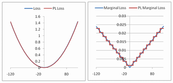
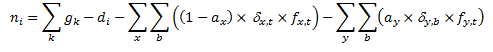
Each loss tranche has an associated (constant) marginal loss equal to the derivative w.r.t. flow of the original quadratic loss function at the mid-point of the tranche. The above figures illustrate for example Line "2_5", the fit to the loss function and the resulting stepwise marginal loss function.
These marginal loss terms appear in the formulation thus: Node Net Injection:
Node Power Balance:
Line Flow Limits:
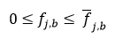
Line Loss Tranche bounds:
where:
- ∑kgk - di is the net generation at node i
- ni is the net injection at bus i (also called the net export)
- x indexes the directed loss tranches exporting from bus i, and
- y indexes the directed loss tranches importing to bus i
- aj is the loss allocation factor for line j
- δj,t is the marginal loss in loss tranche b for line j
- fx,t is the flow in loss tranche b for line j with sets F and B indicating the forward and back directed flows respectively
The optimisation solves these two node balance equations simultaneously. The losses have the effect of being loads at the nodes either end of the line. The nodal price is taken from the dual on the first equation and will naturally include the effect of marginal losses.
We note the following advantages / disadvantages / features of the PL model:
- The resulting formulation is linear and thus can be solved in a single LP problem i.e. no additional iteration is required to 'converge' the loss model;
- and integer programming (MIP) can be added on top with no loss of accuracy.
However:
- The approach will tend to produce flows at corner points of the loss tranches; and
- The marginal loss function is a stepwise linear approximation of the real linear marginal loss function, thus the pricing impact of this approximation is much greater than the absolute error in the loss.
To maximize the accuracy of the marginal loss approximation we can increase the number of loss tranches used. This is controlled with the Transmission Max Loss Tranches or Line Max Loss Tranches. Note that this setting defines the number of loss tranches used in each of the forward and back directions, so a value of five will result in a total of 10 tranches being used across the range of line flows.
It should be noted that marginal loss factor for all tranches are computed based on the lower bound and upper bound of the line. For the case when line flow is allowed to violate out of the limits, the size of the first and last trance are free while the same loss factors are still applied. This approximation is acceptable as in practical network models, the violations of line flow are usually not too faraway from limits. This is for 7.5 version. For 7.6 version, a line is allowed to violate up to 5 times its limit by default when modeling loss & limit penalty. If higher violation is desired, Line.OverloadMaxRating can be used to define the highest possible value.
Non-physical Losses
A potential problem with the piecewise linear model is its assumption that the problem is entirely separable i.e. each loss tranche is a separate decision variable and there is no in-built logic to force them to be taken up in flow order.
In normal circumstances the optimization will want to minimize losses and so it will flow on low loss tranches first before using higher loss ones. But it can occur that there is over-generation (dump energy condition) due to constraints such as generator must-run constraints, system security constraints, or other constraints that force flows or generation against economic dispatch.
When dump energy occurs the nodal prices will be at or below the price of dump energy (set by Region Price of Dump Energy).
The optimization then prefers to maximize losses near the node and will choose the highest loss tranches first. Thus the modelled loss will exceed the losses defined by the original quadratic loss function. These additional losses are what are referred to as non-physical losses (NPL).
Solutions with NPL exhibit one or both of the following symptoms:
- Directional flow variables are chosen for both forward and backward flow directions simultaneously.
- Loss tranches are chosen in 'reverse order' i.e. tranches with higher loss are chosen before those with lower loss.
These solutions clearly have no physical representation, hence the term non-physical losses. In a PLEXOS solution, non-physical losses show up as periods where one or more lines reports very high losses relative to flow.
This problem occurs in all linear programming (LP) based market clearing engines that use piecewise linear loss functions e.g. New Zealand, Australia, Singapore, and Ireland. PLEXOS includes a procedure for correcting non-physical losses as they occur, using integer programming, and this is described in the property Transmission Detect Non-physical Losses.
Quadratic
A quadratic constraint is formulated for each line that represents the line's losses. The formulation is made so that the line loss constraints are conic in nature, which allows the solvers to use interior point methods to solve the problem.
In addition, so solvers that support it, can model integer decisions at the same time as these quadratic constraints (called quadratically-constrained integer programming). This loss model, with its variable shift factors and quadratic losses is the most accurate OPF model available in PLEXOS, but it is also the most computationally difficult.
7. Losses Embedded in the Load
The OPF has fundamental equations that balance supply and demand. For the FS-OPF there is a single system-wide balance equation, and for the VS-OPF there exist the same equations for every node in the network. For convenience, we will discuss the FS-OPF here, but the same applies to the VS-OPF.
Losses are included in the system-wide energy balance constraint thus:
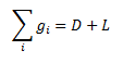
where:
- i indexes nodes
- D is the system demand
- gi is the generation at node i
- L is the system wide losses
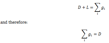
This means that the input demand must agree with:
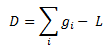
i.e. the input demand must not include transmission losses.
However, in most systems load forecasts are based on generation (which is more convenient to meter than customer load). Therefore the demand input to PLEXOS must be adjusted downwards to account for transmission losses. Alternatively, you can ask PLEXOS to do this automatically during the simulation. The property Transmission Load Includes Losses (yes/no) activates an algorithm that iterates on an adjustment to the demand, converging such that:
You can control the number of iterations used to gain convergence with the Transmission Max Embedded Loss Iterations. If you plan to use this automatic method be sure to check the computational overhead of running it (which is usually light but can vary depending on the loss model) versus the accuracy gained compared to simply scaling the input load down by an estimate of losses in the input data. Note that you can use the load scaling property Region Load Scalar to scale loads automatically, which is often more convenient than modifying the raw input load files.
8. Special Loss Functions
PLEXOS supports defining completely custom line loss functions in three ways:
- By using multiple tranches of flow and incremental loss i.e. a custom piecewise linear loss function; or
- By specifying the terms of a quadratic equation, which can include constant, linear and quadratic terms; or
- By defining a marginal loss factor equation.
Piecewise Linear Functions
Custom piecewise linear loss functions are used in LP-based markets like New Zealand. The line properties Max Flow and Loss Incr and Min Flow and Loss Incr Back can be used in multiple bands (tranches) as shown in Table 4.
Table 4: Custom piecewise linear loss function
| Line | Property | Value | Units | Band |
|---|---|---|---|---|
| 1_2 | Max Flow | 100 | MW | 1 |
| 1_2 | Max Flow | 100 | MW | 2 |
| 1_2 | Max Flow | -100 | MW | 1 |
| 1_2 | Max Flow | -100 | MW | 2 |
| 1_2 | Loss Incr | 0.02 | MW/MW | 1 |
| 1_2 | Loss Incr | 0.025 | MW/MW | 2 |
| 1_2 | Loss Incr Back | 0.02 | MW/MW | 1 |
| 1_2 | Loss Incr Back | 0.025 | MW/MW | 2 |
These data define a piecewise linear loss model with two tranches in each flow direction. The marginal loss for the first tranche is 0.02 = 2%, and for the second tranche 2.5%. Each tranche is 100 MW in size i.e. the [Max Flow] values in each band (tranche) are treated as incremental.
Custom Quadratic Loss Equations
Custom quadratic loss equations can be defined individually for flows in the reference and counter-reference direction as in Table 5 and Figure 3.
Table 5: Custom quadratic loss function
| Line | Property | Value | Units | Band |
|---|---|---|---|---|
| 1_2 | Max Flow | 1000 | MW | 1 |
| 1_2 | Min Flow | -800 | MW | 1 |
| 1_2 | Loss Base | -5 | MW | 1 |
| 1_2 | Loss Incr | 0.01234 | MW/MW | 1 |
| 1_2 | Loss Incr2 | 0.0001234 | MW/MW2 | 2 |
| 1_2 | Loss Base Back | -5 | MW | 1 |
| 1_2 | Loss Incr Back | 0.02345 | MW/MW | 2 |
| 1_2 | Loss Incr2 Back | 0.0002345 | MW/MW2 | 2 |
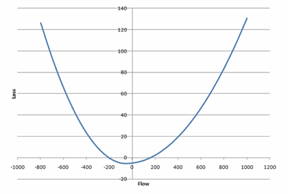 Figure 3: Custom quadratic loss function
Marginal Loss Factor Equations
Marginal loss factor equations describe losses as a function of line flow as well as system demand. They are used in the Australian NEM. PLEXOS supports MLF equations directly through the MLF class.
9. Approximating Losses Using a Penalty Function
In the lossless model the optimal solution may show some transmission lines (particularly DC lines) operating at the extremes of their flow limits. In reality the higher the flow level the higher losses are incurred. One way to moderate the behaviour of the lossless optimization without the overhead of full loss modelling is to impose a quadratically increasing penalty to flows to mimic losses.
This type of penalty function can be synthesized by creating a Constraint with multiple penalty tranches as in Table 6.
Table 6: Penalty function
| Membership | Property | Value | Units | Band |
|---|---|---|---|---|
| DC LOSS | Sense | ≥ | - | 1 |
| DC LOSS | RHS | 0 | - | 1 |
| DC LOSS | Penalty Quantity | 192 | MW | 1 |
| DC LOSS | Penalty Quantity | 192 | MW | 2 |
| DC LOSS | Penalty Quantity | 192 | MW | 3 |
| DC LOSS | Penalty Quantity | 192 | MW | 4 |
| DC LOSS | Penalty Quantity | 192 | MW/MW | 5 |
| DC LOSS | Penalty Quantity | 192 | MW/MW | 6 |
| DC LOSS | Penalty Quantity | 192 | MW/MW | 7 |
| DC LOSS | Penalty Quantity | 192 | MW/MW | 8 |
| DC LOSS | Penalty Quantity | 192 | MW/MW | 9 |
| DC LOSS | Penalty Quantity | 192 | MW/MW | 10 |
| DC LOSS | Penalty Price | 0.07 | MW | 1 |
| DC LOSS | Penalty Price | 0.29 | MW | 2 |
| DC LOSS | Penalty Price | 0.66 | MW | 3 |
| DC LOSS | Penalty Price | 1.18 | MW | 4 |
| DC LOSS | Penalty Price | 1.84 | MW/MW | 5 |
| DC LOSS | Penalty Price | 2.65 | MW/MW | 6 |
| DC LOSS | Penalty Price | 3.61 | MW/MW | 7 |
| DC LOSS | Penalty Price | 4.27 | MW/MW | 8 |
| DC LOSS | Penalty Price | 5.97 | MW/MW | 9 |
| DC LOSS | Penalty Price | 7.37 | MW | 10 |
| Constraint (DC LOSS).Lines (DC) | Flow Coefficient | 1 | - | 1 |
The constraint sense is equality (value=0) and right-hand side is zero. The line's flow coefficient is set to one. The penalty function is entered as multiple bands with increasing penalty. This in fact creates a piecewise linear penalty function which is suitable for the linear optimization used in PLEXOS. Thus the constraint is formulated as:
Minimise
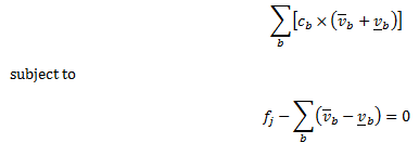
where:
- fj is the flow on line j ins the reference direction (free variable)
- vb is the violation above zero flow in penalty tranche b
- vb is the violation below zero flow in penalty tranche b
- cb is the penalty for flow in penalty tranche b
The penalty function has the desired effect of mitigating extreme flow levels that would in reality incur high losses.