Fuel Optimization with Constraints

Aurora’s Fuel Optimization with constraints can optimize the dispatch of generators subject to fuel limits. This capability is very flexible and can accommodate generators than can burn multiple fuels and multiple generators that burn the same fuel.

One application is for locations with natural gas plants that can only access one or two gas pipelines and have either physical or contractual limits on how much gas they can burn from a given pipeline. However, this logic can easily be applied more broadly including to multiple fuel types and provides a convenient framework from which changes in fundamentals may be analyzed and more generally considered.

In brief, the fuel optimization logic employs a Linear Program (LP) methodology to find a dispatch pattern that minimizes system production cost over the day or hour in which the limit applies.

This document consists of:

A description of input data requirements and output results available
Setup guidelines to use this feature effectively
Additional clarification of how to and how not to employ “nesting” of multiple fuels per generator
A tutorial based on a real-world example in Florida
A brief description of other important considerations

Input Assumptions and Output Results

Input Data Requirements

Fuel input table:

Reference Fuel column – Allows any given fuel to reference (or depend on) other source fuels. Multiple reference fuels may be specified in a comma separated list.
Daily Fuel Limit column - If this value >= 0 for any fuels used in the system, then the Fuel Optimization logic will be invoked for the dispatch. If left blank, no limit is applied. It is specified in the same units as the Fuel Units column for each fuel (e.g. mmBtu by default). All resources that utilize this fuel directly or indirectly (via a Reference Fuel) will be cumulatively limited to this amount per day.
Hourly Fuel Limit column - If this value >= 0 for any fuels used in the system, then the Fuel Optimization logic will be invoked for the dispatch. It is specified in the same units as the Fuel Units column for each fuel (e.g. mmBtu by default). All resources that utilize this fuel directly or indirectly (via a Reference Fuel) will be cumulatively limited to this amount per hour.

Output Data Results

FuelDay, FuelHour tables:

Referenced_Usage – This column reports the total fuel used for a given fuel, for every resource that directly uses or indirectly references this fuel. By contrast, Usage only reports the fuel directly used (i.e. this fuel’s ID must be present in the Fuel column of the Resources table for at least one resource). This value is reported in the same units as Fuel Units for this fuel in the Fuel table of the input database (default is mmBtu).
Input_Limit– This value in the FuelDay or FuelHour output tables mirror what was entered in the Daily Fuel Limit andHourly Fuel Limit columns, respectively, if the input Fuel table.
Limit_Shadow – This value (currency per heat-rate heat content, typically $/mmBtu) represents the value of the constraint. In other words, if we increased the fuel limit by one unit (1 mmBtu), what reduction in total system production cost could we expect ($)? Hence, the higher the shadow price, the more binding the constraint. As expected, when the Usage < Input_Limit, then the Shadow Price = 0.

Setup For Fuel Optimization

In order to understand how to best set up a fuel optimization run, it is helpful to consider the answers to three fundamental questions:

Over what scope are the fuel limits binding?

In other words, is the fuel limited at the source pipeline level? Or to an individual generating unit? Or to a set of generating units (e.g. plant level)? Or all of the above?

What are the unique fuels available to those generating resources?

If any of the modeled generators can burn multiple fuels (especially when a primary or alternative fuel supply is limited), then those fuel options need to be identified for each generator.

At what level of detail do I want fuel usage reporting?

Aurora is very flexible in the ability to define individual fuels (used by generators) in terms of ‘reference fuels’ and those can be cascaded together into appropriate chains.

For example, assume that many generators—including generator_1—can burn gas from pipeline_A or pipeline_B, and that there are daily limits for both pipelines, but hourly limits at the plant affecting generator_1. Further, assume that we want to know how much fuel from pipeline_A and from pipeline_B was burned by generator_1 in each time period. In addition, a daily fuel limit on Fuel A with value x says that the total fuel used by all resources burning fuel from pipeline_A in the given day must be less than or equal to x.

Multiple Fuel Setup and Nesting

Q: How to specify a generator’s ability to burn fuel from multiple sources (which may or may not be limiting)?

In the Reference Fuel column of the Fuel input table, you can enter as many unique fuel sources as desired (comma separated). So, generator_1 can be assigned to burn a fuel called fuel_gen1, and fuel_gen1 is assigned multiple reference fuels: pipeline_A, pipeline_B, pipeline_C,etc.

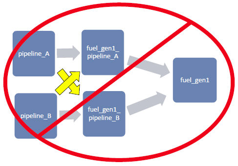
However, in this case, total fuel burn by the pipeline is reported as well as total fuel burn by generator, but it does not break out how much fuel from each pipeline is burned by each generator. To accomplish this, a nested structure is required.

Now add two fuels to be defined: fuel_gen1_pipelineA, and fuel_gen1_pipelineB. (NOTE: these are not physical fuels, but merely Fuel IDs specified for convenience in defining and reporting.) Fuel_gen1 references fuel_gen1_pipelineA and fuel_gen1_pipelineB, and those, in turn, reference pipeline_A and pipeline_B, respectively.

This type of nesting or cascading references is allowed—even multiple times—so long as those fuel references do not attempt to reference multiple fuels themselves.

Tutorial

Much of the state of Florida is limited in its ability to import natural gas via two pipelines: Florida Gas Transmission Company, LLC (FGT), Gulfsteam (GS).

Sources:

Panhandle Energy, http://www.panhandleenergy.com/comp_fld.asp

Gulfstream Natural Gas, http://www.gulfstreamgas.com/

Assume we want to optimize the Florida Power & Light (FPL) system’s natural gas fuel burn given daily limits on those two pipelines and hourly limits at the power plant level, specifically the Manatee units.

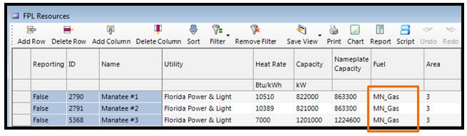
Step 1 – Assign Fuels

Define a fuel for those units to burn, in this case MN_Gas, and assign each of the 3 units to burn that fuel in the Resources table as shown in the figure below.

Step 2 – Create Fuels

We then go to the Fuels table and specify five fuels: FGT is pipeline 1, GS is pipeline 2, FGT_to_Manatee and GS_to_Manatee reference these first two fuels (placeholders described below), and finally MN_Gas, which references both FGT_to_Manatee and GS_to_Manatee. This last fuel, MN_Gas, represents the portions from FGT pipeline and from GS pipeline that feed the plant and was assigned to the resource in step 1.

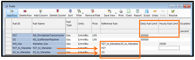
The two intermediary fuels, FGT_to_Manatee, and GS_to_Manatee, are not physically limited. They are simply structural placeholders for reporting purposes so we can easily get output reporting of how much fuel usage (mmBtus) came from pipeline 1 (FGT) vs. pipeline 2 (GS) at Manatee. At the top of the food chain, we have the pipelines themselves, FGT and GS, and we can place daily (or hourly) limits on those as appropriate as in figure above.

Step 3 – Setup More Fuels

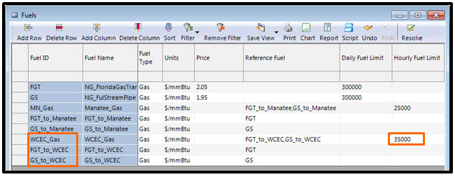
We can then expand this structure to as many gas units as we need to. The figure below shows the addition of plant level fuel WCEC_Gas, which has an hourly limit of 35,000 mmBtus. It references two intermediate fuels FGT_to_WCEC and GS_to_WCEC, which in turn reference FGT and GS, just as MN_Gas does.

Step 4 – Run

If daily or hourly fuel limits >= 0 are specified for any fuels used in the system, then the Fuel Optimization logic will be invoked for the dispatch. If none of the fuel limits are ever binding, then the results will be as if no limits were identified in the first place. Ensure you have Daily or Hourly reporting for Fuel output selected.

Step 5 – Observe Output

In the FuelDay table, which reports daily fuel output, we can easily see the fuel burn at the generating unit level, including the contributions from each constituent pipeline as shown in figure below.

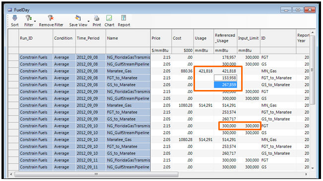
We can verify that the Referenced_Usage of the Manatee Gas components, FGT_to_Manatee and GS_to_Manatee, sum to the Manatee total Manatee_Gas. We can also compare the Referenced_Usage for any fuel that has a daily limit (Input_Limit) to ensure it is never exceeded (300,000 mmBtus in figure above).

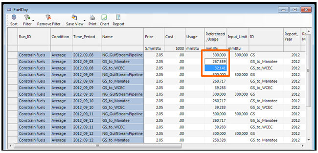
Likewise, we could sum up all Referenced_Usage for “GS_to_xxx” components to see that they total NG_GulfStreamPipeline(GS) as show in figure below. In this example, two generators, Manatee and WCEC, are tied to NG_GulfStreamPipeline.

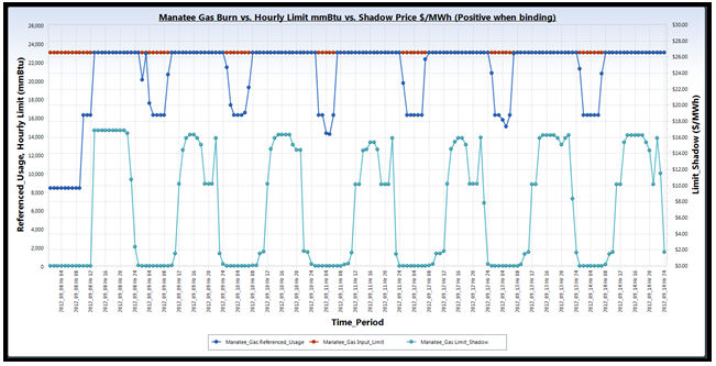
Finally, we can verify that the hourly limits at the generator level were also honored, and how much each pipeline is contributing to the total fuel burn in each hour at that plant. See figure below.

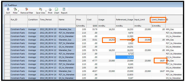
Note also, in the figure above, the Limit_Shadow column which reports a shadow price on the constraint. It represents the change (lowering) in system cost (e.g., $) for every increase (relaxing) of the fuel limits by 1 unit (e.g. mmBtu). Hence, the higher the shadow price, the more binding, the constraint.

As expected, this happens during the on-peak hours. Conversely, during the off-peak hours the Usage is less than the Input_Limit and the resulting Shadow Price = 0. See figure below.

Other Considerations

Daily vs. Hourly Optimization – When running with daily limits, the model needs to resolve all data for the day before it can solve the dispatch for each hour. Because of this, the commitment optimization logic (which solves the dispatch for all hours of the day simultaneously) must be employed with daily limits.

Daily Limit Scaling with Sampling – The daily limits should always be input for the full day, even when running sampled hours. The model will automatically scale the daily fuel limit as needed to account for the effect of sampling. For example, if the total daily fuel limit for a given fuel is input as 100,000 mmBTU and the simulation is only sampling every other hour, then the model will automatically set the total limit for the 12 hours being dispatched to 50,000 mmBTU.

Monthly Limits – Daily fuel limits are not compatible with nonzero monthly fuel limits for primary and/or secondary fuels in the Resources table. Monthly fuel limits of zero specified through the Time Series Monthly table may still be applied to preclude the use of a primary or secondary fuel for certain months.

Infeasibilities – To ensure that infeasibilities in the LP do not occur, users should always ensure that there is plenty of unconstrained capacity in each zone. Typically, this is done by including a large MW amount of demand curtailment which can be used to dispatch as a last resort when physical resources have been exhausted.

Time Series – The hourly and daily fuel limits may be input using the time series logic, so the values can change yearly, monthly, or daily. The hourly limits can also change on an hourly basis using the Time Series Weekly or Time Series Hourly tables. For more information on how to specify a time series for a variable, see Entering a Time Series.

Tutorials

Fuel Optimization With Constraints