Combined Cycle
Contents
- Introduction
- Waste Heat Transfer and Efficiency
- Unit Commitment and Outages
- Duct Burner
- The Example Solved
- Ancillary Services
- Heat Load and District Heating
- Modelling CCGT Using Heat Node
- Modelling CCGT Configuration
1. Introduction
PLEXOS models combined-cycle plant by explicitly tying the waste heat output of one or more units to the heat input of another unit. Specific features available in this model include:
- Waste heat from units of different size and efficiency.
- Accounting for boiler efficiency.
- Steam- turbine heat rate as a function of loading level.
- Duct- burner model.
- Exogenous steam loads e.g. for loads associated with co-generation plant.
The PLEXOS combined-cycle model is shown in Figure 1. In this representation:
- CT units are represented by generator objects (either one for each CT or a multi-unit Generator).
- The boiler, duct burner and steam turbine (ST) are represented by a single generator object.
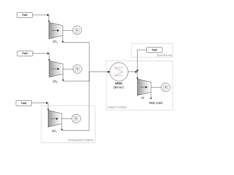 Figure 1: Combined Cycle Model
this article follows and example based on a 2 x 1 setup with the
following characteristics:
- There are two CT units with capacities of 160 MW each.
- The CT heat rate is described by a marginal heat rate function of five steps.
- The boiler efficiency is 80%
- The single ST unit has a capacity of 140 MW with a single constant heat rate
- The unit can fire a duct burner to provide another 50 MW
Table 1 presents the CT unit data for this case, Table 2 the ST data. For the example, assume there are two identical CT units (CT1 and CT2).
| Property | Value | Units | Band |
|---|---|---|---|
| Units | 1 | - | 1 |
| Max Capacity | 160 | MW | 1 |
| Min Stable Level | 160 | MW | 1 |
| Heat Rate Base | 200 | MMBTU | 1 |
| Heat Rate Incr | 8000 | BTU/kWh | 1 |
| Heat Rate Incr | 8800 | BTU/kWh | 2 |
| Heat Rate Incr | 9600 | BTU/kWh | 3 |
| Heat Rate Incr | 9800 | BTU/kWh | 4 |
| Heat Rate Incr | BTU/kWh | BTU/kWh | 5 |
| Load Point | 64 | KW | 1 |
| Load Point | 88 | MW | 2 |
| Load Point | 112 | MW | 3 |
| Load Point | 136 | MW | 4 |
| Load Point | 160 | MW | 5 |
| Min Up Time | 4 | hrs | 1 |
| Min Down Time | 2 | hrs | 1 |
| Property | Value | Units | Band |
|---|---|---|---|
| Units | 1 | - | 1 |
| Max Capacity | 190 | MW | 1 |
| Min Stable Level | 0 | MW | 1 |
| Boiler Efficiency | 80 | % | 1 |
| Heat Rate | 12700 | BTU/kWh | 1 |
Note carefully that the ST total capacity is the sum of the 'normal'
capacity plus duct burner capacity - we will discuss how to limit the
duct burner contribution below.
Assume that a fuel called GAS has been defined. Given this, the
relevant memberships for the combined-cycle plant are shown in Table
3. All three generating units use GAS (Point 1 in ). Note that the ST
need not have a fuel membership because it receives waste heat from
the CTs via the boiler, but this is included to model the duct-burner
facility (Point 2 in ) i.e. the fuel burned by the ST will represent
the duct burner use, with efficiency adjusted according to the boiler
efficiency.
| Collection | Parent Name | Child Name |
|---|---|---|
| Generator Fuels | CT1 | GAS |
| Generator Fuels | CT1 | GAS |
| Generator Fuels | ST | GAS |
| Generator Heat Input | ST | CT1 |
| Generator Heat Input | ST | CT2 |
For clarity, this example is deliberately simplified, so it is
important to note that you have access to all the usual generator
modelling features for each of the CT and ST units and there are no
preset limits on the configuration (2 × 1, 3 × 1, 4 × 1, etc).
2. Waste Heat Transfer and Efficiency
Waste heat is 'transferred' from one generator to the next using the
Generator Heat Input collection. In our example the ST unit takes
waste heat from both CT1 and CT2 as defined by the memberships in
Table 3.
The amount of heat transferred from the CTs to the boiler is equal to
the fuel input to the CTs less the electric output of the CTs (at
notional maximum efficiency). Note that you should choose the
appropriate metric or imperial units model (under Settings in PLEXOS)
so that the efficiency conversion is computed consistent with the
input heat model e.g. Using 100% efficiency equals 3.6 fuel units per
megawatt hour in metric or 3.412 in imperial.
The waste heat is then passed through the boiler before being used in
the ST. The boiler is modelled as part of the ST and its efficiency is
defined using the Boiler Efficiency property e.g. 80%. By default this
efficiency is 100%.
The ST unit will produce electric output from the steam output of the
boiler according to its heat rate i.e. the steam input acts just like
a 'free' fuel source. The waste heat produced by ST is the remaining
energy after generation, which is defined differently from the input
waste heat. (See Waste Heat)
Additional fuel can be injected to the boiler (duct burner facility)
as described below.
3. Unit Commitment and Outages
The ST unit cannot operate unless at least one of the CT units is
operating. PLEXOS automatically enforces this rule when the Generator
Heat Input membership is defined between the units.
Generator outages may be modelled on CT and ST units in the usual
manner - as described in [2]. Because PLEXOS explicitly models heat
transfer the overall efficiency of the combined-cycle plant will
correctly account for the number of CTs on-line and the heat rate as a
function of the CT and ST units.
When all CT units are out of service the ST will not operate, however
the CT units may operate independently of the ST - but would only do
so if the price they receive is high enough to at least compensate
them at their raw CT heat rate.
4. Duct Burner
Some combined-cycle plant can boost generation from the ST part by
injecting fuel into the ST. This duct burner facility is modelled in
PLEXOS by adding a fuel membership to the ST unit, as in Table 3.
By default the duct burner capacity would be limited only by the ST
capacity so we use the property Generator Fuels Max Input to set a
limit on the fuel injected into the duct burner, as in Table 4. The
figure of 625 is the ST heat rate multiplied by the 50 MW capacity of
the duct burner.
Note that the fuel injected at the duct burner enters AFTER the boiler
and thus is NOT subject to the efficiency of the boiler component.
| Membership | Property | Value | Units |
|---|---|---|---|
| Generator (ST) Fuels (GAS) | Max Input | 625 | MMBTU |
5. The Example Solved
Need to provide example database for this case.
Now assume that the combined-cycle plant generates into an external
energy market with an uncertain forward price. The illustrations below
present a selection of the results from a sample week.
Referring to Figure 2 it is clear that the automatic logic constraints
that PLEXOS produces that control when the steam turbine can operate
are in force; also the steam turbine output varies according to how
much waste heat is coming from the CT units, and this is a function of
their loading level and heat rate. The noticeable spike in ST output
during high priced periods Figure 3) is produced by the duct burner
capability and this is easily seen from the fuel offtake results
(Figure 4) in which the ST unit only uses fuel when it is utilizing
the duct burner facility.
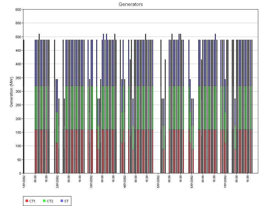 Figure 2: CCGT Generation by Unit
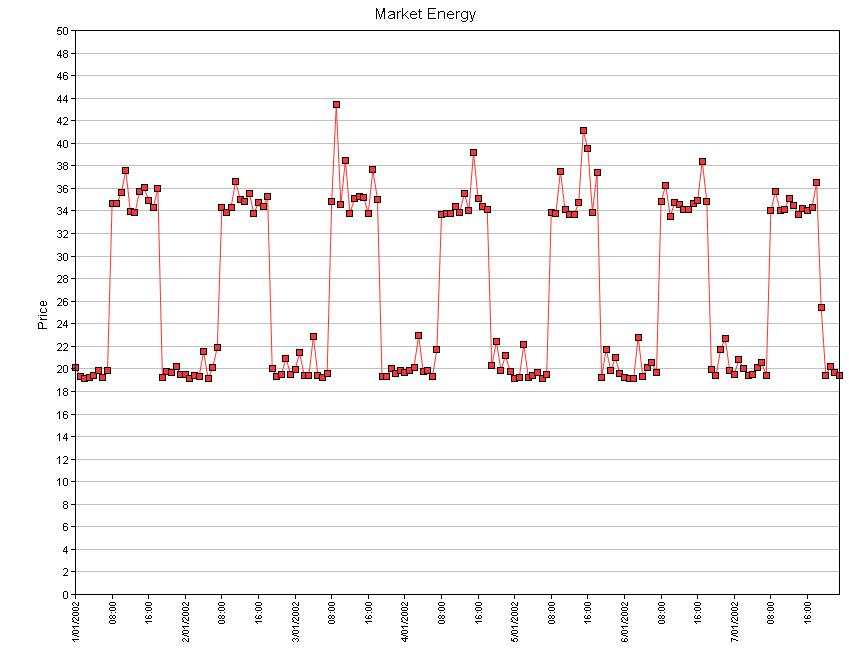 Figure 3: Energy Market Prices (endogenous stochastic variable)
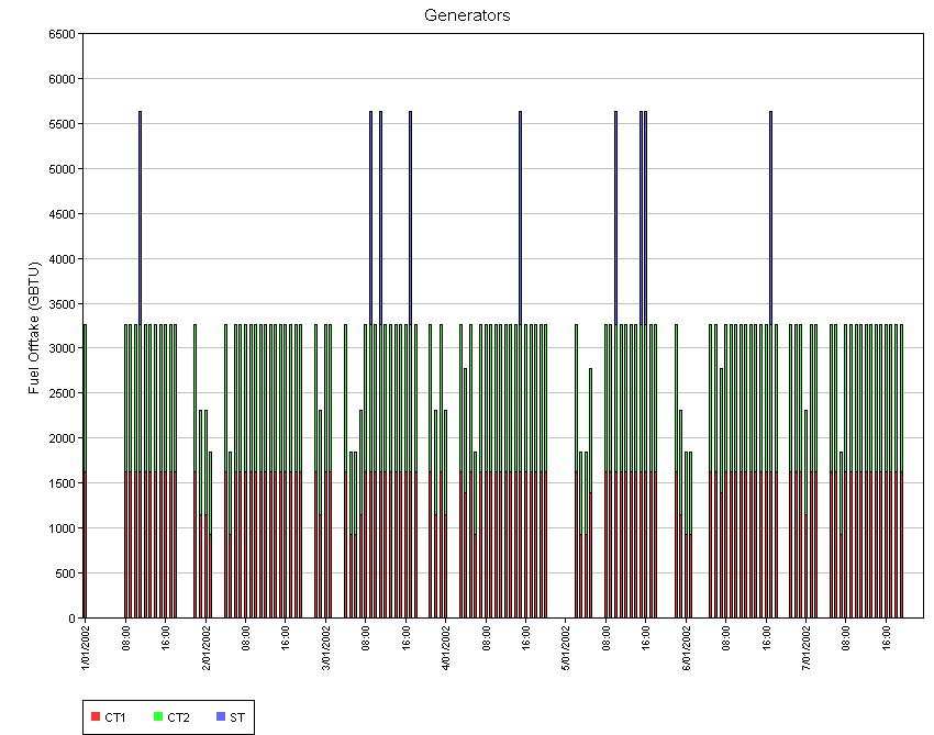 Illustration 3: CCGT Fuel Use by Unit
6. Ancillary Services
Both CT and ST units may provide reserve-as described here.
7. Heat Load and District Heating
An exogenous heat load can be placed on the ST unit using the
property Heat Load described in [4], and this is useful for modelling
co-generation plant. This load will always be met if physically
feasible.
PLEXOS can also arbitrage optimally between electric production and
supply of heat to an external heat market (which might represent a
contract to supply district heating for example)-these options are
described in Market class.
8. Modelling CCGT Using Heat Node
Another alternative way to model the CCGT from PLEXOS 7.6 version is using the new heat class feature. GT generators are connected to a heat node via Heat Output Nodes membership. ST generators are linked to the same heat node via Heat Input Nodes membership. The auxiliary boiler can be modelled by the Heat Plant class. See Heat Modelling for more details.
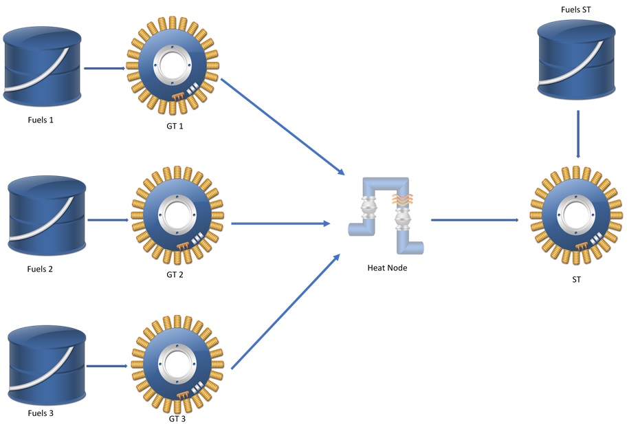 Figure 4: Model CCGT using heat class.
Modelling CCGT Configuration
When there are 2 or more GT generators connecting to a same ST
generator (or even more ST), there exists several CCGT configurations
or combinations. For example, 1 GT runs with the ST or 2 GTs runs
parallel with ST. Currently, PLEXOS does not model the configuration
specifically. However, it can be achieved using the Generic
constraints and Decision Variables. This section presents an example
on how to model the CCGT configuration for 3 GT and 1 ST. Please
contact Energy Exemplar staff for a copy of the example model.
In this example, we model 3 GT and one ST. There are 3 possible
configurations for this CCGT operation.
- GT1Alone : Run only GT1; GT2 and GT3 are not running.
- GT1>2 : running GT1 and GT2; GT3 is not running
- GT1&G1&G3: running 3 GTs
9.1 Decision Variables:
Creating 3 decision variables (called GT1alone, GT1+GT2, GT1+G2+GT3). They are all binary decision variables (Type = Integer, Lower bound = 0, Upper Bound = 1).
9.2 Generic Constraints:
- Configuration GT1 Alone:
GT1Alone = [UnitGeneratingCoefficient]_GT1
G1Alone + [UnitGeneratingCoefficient]_GT2 =< 1
G1Alone + [UnitGeneratingCoefficient]_GT3 =< 1
- Configuration GT1>2>3
GT1>2>3 =< (UnitGeneratingCoefficient]_GT1 +
UnitGeneratingCoefficient]_GT2+ UnitGeneratingCoefficient]_GT3)/3
GT1>2>3 =< (UnitGeneratingCoefficient]_GT1 +
UnitGeneratingCoefficient]_GT2+ UnitGeneratingCoefficient]_GT3) - 2.99
- Only one configuration state is allowed.
GT1Alone + GT1Alone + (GT1>2) + (GT1>2>3) =< 1
With the above constraints and decision variables, we can know which
configuration is active.
9.3 Special Technical Constraints
If there is any special CCGT configuration rule required, additional
constraints can be added using the above decision variables.
For example, we can't move from state GT1>2>3 to GT1alone
and vice versa. In this case, we need to write this constraint (using
time lag)
GT1Alone(t-1) + GT1>2>3(t) =<1
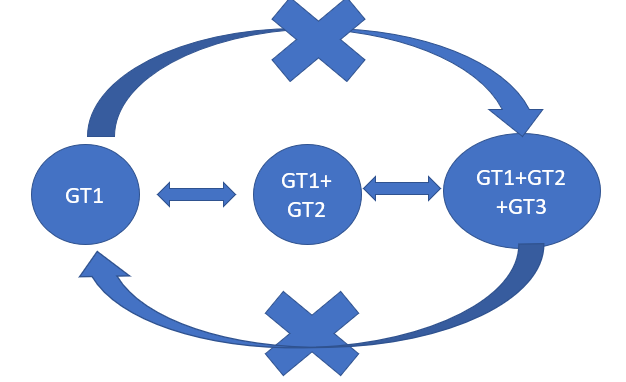 Figure 5:Configuration Rule.
Another common requirement is modelling the transition time from one
configuration to another. For example, the transition from state
GT1Alone to GT1>2 is 45 minute. First of all, we need to know
the number of intervals covering the transition time. N = [Transition
Time]/[Interval length]. Says the simulation interval is 15 minute, we
have N = 45/15 = 3 Using the time lag feature, we will write N generic
constraints as:
GT1Alone(t) + GT1>2(t) =< 1 (1)
GT1Alone(t) + GT1>2(t+1) =<1 (2)
...
GT1Alone(t)+ GT1>2(t+N) =<1 (N)
This means that if GT1Alone is active, the next 3 intervals (45
minutes), state GT1>2 cannot be used.
References