Cascading Hydro Networks

Contents

1. Introduction
2. The Potential Energy Model
3. Hydro Generator Efficiency
4. The Level Model
5. The Volume Model
6. Hydraulic Connections in a Cascade
7. Hydro Visualization Tools

1. Introduction

The previous chapters of this article dealt with 'stand alone' storages or simple 'closed circuit' pumped storage systems. In those systems the conversion of water to electrical energy is a static function and thus storage volumes can be expressed in units of potential energy (GWh)

2. The Potential Energy Model

When one considers a cascade of storages with multiple generators, however, the potential energy in the system is not simply a function of the total volume of water in the system, but also of which storages are holding that water. Consider a system with two storages and identical generators in a linear cascade like Figure 1. On the left the upper storage is full, the lower is empty and vice versa on the right. The potential energy in the left-hand system is double that of the right-hand system. This is because water stored in the upper storage can generate in both the upper and lower generators, whereas water in the lower storage can only generate in the lower generator.

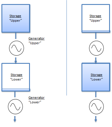Figure 1: Simple cascade

Again if this system remains "static" it can still be modelled in PLEXOS as a potential energy network. All that is required is to express the volume of the upper storage in terms of potential energy for the entire cascade, and then apply a scaling factor that "derates" that potential energy once it passes through the upper generator.

In fact hydro efficiency can vary even in a single storage model due to head effects: efficiency varies as a function of the difference in heights of the head and tail storages which varies as those storages are filled/emptied.

once it passes through the upper generator. PLEXOS provides the properties Generator Head Storage Flow Factor and Generator Tail Storage Flow Factor for just this purpose.

However if at any time one of the generators in the cascade goes out-of-service the simplistic scaling of potential energy will not be accurate. Further, if the cascade is anything but a linear system, e.g. if multiple sources feed a storage, then again the potential energy model is not accurate. Thus PLEXOS provides alternate hydro models that work on raw volumes of water for storage and directly model generator efficiency.

3. Hydro Generator Efficiency

In the Level and Volume models in metric mode, hydro generator efficiency is expressed in megawatts per cubic meter second (MW/cumec) i.e. it is the rate of production that results from a flow rate through the turbine of one cubic meter per second. This efficiency is input via the property Generator Efficiency Incr.

Hydro generator efficiency is allowed to vary according to the generation level by using Efficiency Incr in multiple bands with Load Point, usually in combination with the "intercept" term Efficiency Base. An example is shown in Figure 2 (in metric units).

PLEXOS develops a piecewise-linear approximation to the efficiency function, and this is illustrated in Figure 2 (showing flow rates) and Figure 3 (showing volumes of water through the turbine per hour).

Table 1: Hydro efficiency curve (metric)

Property	Value	Units	Band
Units	1	-	-
Max Capacity	60	MW	-
Load Point	20	MW	1
Load Point	40	MW	2
Load Point	60	MW	3
Efficiency Base	58	cumec	-
Efficiency Incr	0.5	MW/cumec	1
Efficiency Incr	0.48	MW/cumec	2
Efficiency Incr	0.42	MW/cumec	3

Table 2: Hydro efficiency curve (imperial US)

Property	Value	Units	Band
Units	1	-	-
Max Capacity	60	MW	-
Load Point	20	MW	1
Load Point	40	MW	2
Load Point	60	MW	3
Efficiency Base	58	cumec	-
Efficiency Incr	0.5	MW/cumec	1
Efficiency Incr	0.48	MW/cumec	2
Efficiency Incr	0.42	MW/cumec	3

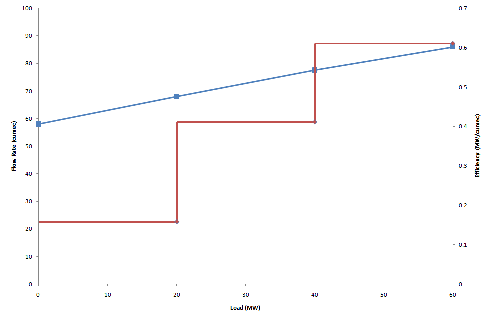
Figure 2: Generator efficiency - flow rate and piecewise linear incremental efficiency (metric units)


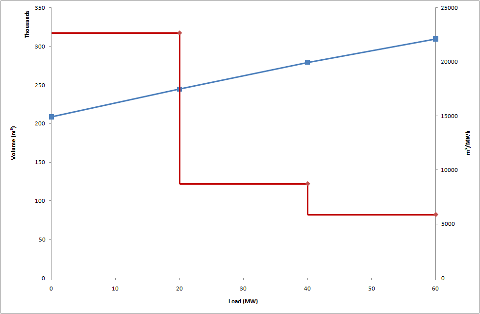
Figure 3: Generator efficiency - water volume and piecewise linear incremental efficiency (metric units)

4. The Level Model

Storages in the Level Model define their capacity using two pairs of elevation and area measures expressed as these Storage properties:

• Low Ref Area, Low Ref Level: the surface area and elevation for 'low' storage
• High Ref Area, High Ref Level: the surface area and elevation for 'high' storage

It is important to note that these pairs are only used to define the storage shape as illustrated in Figure 4. The additional properties Min Level and Max Level define the feasible range of storage levels allowed: these need not be within the Low Ref Level and High Ref Level range. If preferred these limits can be defined using Min Volume and Max Volume where zero volume is defined at the Low Ref Level.

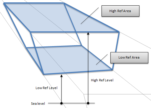Figure 4: Level Model parameters

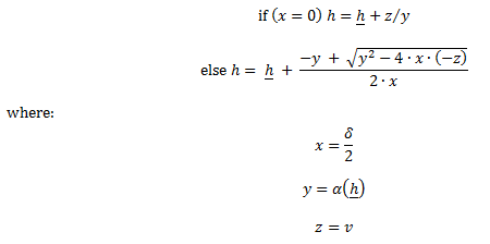
PLEXOS converts the level information to volumes for use in the storage optimization and in interpreting and reporting volume-based limits and solution values. Given the reference pairs, the volume in the storage v equivalent to a given level h is computed using the formula:

and:

h is the Storage Min Level (minimum defined in entire horizon)
a* and a* are the Storage Low Ref Area and High Ref Area respectively
h* and h* are the Storage Low Ref Level and High Ref Level respectively

The volume in storage v can be then converted back to level h by "completing the square":

Case 7

Storage using the level model:

As a demonstration of the Level model and use of hydro generator efficiency, assume we wish to convert the hydro generator with storage in our example developed earlier (Case 3) to one of the same 'size', in terms of potential energy, but defined using level data. For simplicity assume that:

• the storage has straight sides (a=a) and that it has an elevation of 100m when full, zero when empty (h=0,h=100). This means that the total volume in storage is given by v=100•a.
• hydro generator efficiency is constant at 1 MW/cumec

The potential energy in the storage is given by e=v/(3600=(100•^-a)/3600). Solving for the required area given a requirement for 5000 GWh of potential gives:

a=(e•3600)/100=(5 000 000•3600)/100=180 000 000 m2

Note that the factor of 3600 converts the cumec flow rate into an equivalent hourly quantity. Also note the conversion of GWh to MWh. The corresponding Storage input to PLEXOS is shown in Table 3. We must also set Generator Efficiency Incr = 1 for this example.

Table 3: Storage input for Level model

Property	Value	Units
Min Level	0	m
Max Level	100	m
Initial Level	100	m
Low Ref Level	0	m
Low Ref Area	180, 000, 000	m3
High Ref Level	100	m
High Ref Area	180, 000, 000	m3

In the metric Level model Generator Efficiency is defined in units of MW/cumec rather than MWh/MWh implied by the potential energy model. In this example a generator efficiency of unity implies that megawatts and cumec are interchangeable thus we do not need to convert the existing Storage Natural Inflow data i.e. the same nominal values will 'work' as cumec.

The results for this case in terms of thermal production cost and energy prices are identical to Case 3 above. The reported storage results however are now in units reflecting volumes of water as in Table X.

Month	Initial Volume (1000 m3)	Inflow (1000 m3)	Release (1000m3)	End Volume (1000m3)	End Level (m)	Shadow Price ($/1000m3)
Jan	18, 000, 000	1, 261, 526	1, 632, 981	17, 628, 545	98	35.7
Feb	17, 628, 545	1, 376, 525	1, 176, 178	17, 828, 892	99	35.85
Mar	17, 828, 892	1, 491, 869	1, 324, 077	17, 993, 731	100	35.83
Apr	17, 996, 684	1, 607, 040	1, 609, 993	17, 993, 731	100	36.41
May	17, 993, 731	1, 146, 355	1, 140, 086	18, 000, 000	100	45.54
Jun	18, 000, 000	572, 832	1, 212, 855	17, 359, 977	96	50.53
Jul	17, 359, 977	0	1, 416, 630	15, 943, 347	89	50.76
Aug	15, 943, 347	115, 171	1, 369, 490	14, 662, 881	81	51.1
Sep	14, 689, 028	1, 148, 256	1, 174, 403	14, 662, 881	81	49.32
Oct	14, 662, 881	1, 376, 698	705, 187	15, 334, 391	85	50.79
Nov	15, 334, 391	1, 721, 088	240, 416	16, 815, 063	93	50.79
Dec	16, 815, 063	1, 261, 526	76, 590	18, 000, 000	100	51.95

5. The Volume Model

Storages in the Volume Model define their capacity in units of water volume:

• Cumec days (CMD) for the metric model;
• Acre feet (AF) for the imperial model.

As discussed above, the central difference between the Level and the Volume model is the way storage dimensions are defined. The volume model uses the same flow units as the Level model.

Case 8

Storage using the volume model:

A cumec day is the volume of water released in a day at a rate of one cumec (cubic metre per second), thus 1 CMD = 3600 × 24 = 86400m3.

Thus to adapt the Level model example above, we need only divide the cubic metre figures by this amount. This gives the following set of Storage input:

Table 6: Results for Case 8

Property	Value	Units
Min Volume	0	CMD
Max Volume	208333	CMD
Initial Volume	208333	CMD

Storage inflows are in cumec (metric) or acre-feet per hour (imperial). For our example the existing cumec-based Storage Natural Inflow values remain unchanged.

Table 6: Results for Case 8

Month	Initial Volume (CMD)	Inflow (CMD)	Release (CMD)	End Volume (CMD)	Shadow Price ($/CMD)
Jan	208, 333	14, 601	18, 900	204, 034	856.8
Feb	204, 034	15, 932	13, 613	206, 353	860, 46
Mar	206, 352	17, 267	15, 325	208, 261	873.82
Apr	208, 295	18, 600	18, 634	208, 261	873.82
May	208, 261	13, 268	13, 195	208, 333	1, 092.93
Jun	208, 333	6, 630	14, 038	200, 926	1, 212.81
Jul	200, 926	0	16, 396	184, 530	1, 218. 325
Aug	184, 530	1, 333	15, 851	170, 012	1, 226.47
Sep	170, 012	13, 290	13, 593	169, 709	1, 183.664
Oct	169, 709	15, 934	8, 162	177, 481	1, 222. 397
Nov	177, 481	19, 920	2, 783	194, 619	1, 218. 936
Dec	194, 619	14, 601	886	208, 333	1, 246.831

6. Hydraulic Connections in a Cascade

The building blocks of a cascading hydro network are:

• Storage
• Generator
• Waterway
• Initial Storage Position
• Natural Inflows

Generators flow water from their Head Storage to their Tail Storage. Where the Tail Storage is not defined, the water flows 'to the sea'. Thus Generator objects are the primary mechanism for connecting Storage objects in a cascading network. Where a storage connects to one or more others without flowing water through a turbine use the Waterway class. A Waterway flows water from its Storage From to its Storage To. Again, when the Storage To is not defined, the waterway flows water 'to the sea' i.e. it is a 'spill'. The final element is natural inflows, which are defined with Storage Natural Inflow.

Case 9

Hydro cascade system using equivalent formulation:
This example uses a hydro cascade of four storages and four generators as in Figure 5: Cascading Hydro Network.

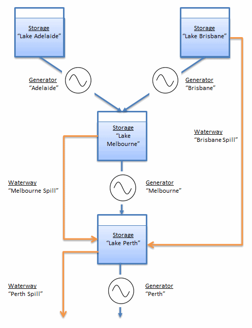Figure 5: Cascading Hydro Network

As the water runs downstream in a cascade system, there is also a loss of potential energy during the trajectory. There are different ways it can be handled in PLEXOS which are related to the hydro model selection. In the case of the energy model, properties Generators Efficiency Incr and Waterway Output Scalar Scalar can be used for that purpose as in the following example.

Table 7: Hydro Generator Efficiency

Generator	Max Capacity MW	Efficiency MW/MW
Adelaide	700	0.68627451
Brisbane	700	0.68627451
Melbourne	220	0.215686275
Perth	100	0.098039216
Thermal	3000	-

First, let's assume we have the following energy data hydro model. In this example, all four storages will try not to run out of water because natural inflows are taken from a deterministic sample. It is also assumed that both upper storages Lake Adelaide and Lake Brisbane have the same amount of natural inflows although they come from independent sources. The rest would take water from the spillways and from the generator releases upstream. Furthermore, spillways don't have delays although they have flowing limits.

Table 8: Waterway Constraints and Output Scalar

Property	Max Volume GWh	Initial Volume GWh	End Effects Method
Lake Adelaide	2900	-	Recycle
lake Brisbane	4600	-	Recycle
Lake Melbourne	1000	500	Recycle
Lake Perth	500	250	Auto

Note that only Lake Perth is allowed to schedule end volume freely End Effects Method='Auto'.

Table 9: Waterway constraints and output scalar

Property	Transversal Time (hrs)	Max Flow	Min Flow	Output Scalar
Spill Brisbane-Perth	0	1000	0	0.098039216
Spill Melbourne-Perth	0	1000	0	0.3125
Spill Perth	0	1000	0

If we take for example 'Lake Adelaide', the result would then show that the end volume for each simulation step must equal the initial value of the next one. Furthermore, the end volume at the end of the simulation (in this case one year) must equal the initial volume as the Generator End Effects Method for storage object 'Lake Adelaide' has been set to 'Recycle'.

Table 10: Results for Case 9. Example of Lake Adelaide Storage Results

Initial Volume (GWh)	End Volume (GWh)	Natural Inflow (MW)	Generator Release (GWh)	downstream Release (GWh)	Generation (GWh)
573.71	653.17	287.93	202.09	0	138.69
653.17	878.6	350.57	133.06	0	91.32
878.6	1098.25	371.3	149.4	0	102.53
1098.25	1276.01	371.3	149.4	0	102.53
1276.01	1235.69	322.47	369.65	0	253.68
1235.01	981.16	171.2	421.6	0	289.33
981.16	543.21	14.78	446.91	0	306.7
543.21	63.78	49.4	516.41	0	354.4
63.78	0	309.92	387.41	0	265.87
0	47.41	406.09	354.15	0	243.04
47.41	331.55	456.28	183.86	0	126.18
331.55	573.71	334.82	85.47	0	58.65

Note that the optimal solution did not require any spillage at any time although releasing water from storages is allowed.

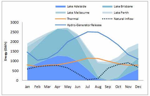Figure 6: Hydro-thermal coordination results for Case9. Energy Model results

Given that this is a deterministic model, the MT scheduler can foresee in advanced the reduction of natural inflows during the months of July and August (dashed line in the figure). The end volumes, for each storage (areas in the figure), drops considerable during the following month. In general, the optimal solution tends to distribute "evenly" the thermal generation avoiding excessive use during the dryer season. However, the risk of optimal deterministic solutions is that minimum end volumes of storages can be binding during water drought stages, leading to aggressive strategy decisions.

Alternative Modelling

Volume Model:
The following example will show how to perform a conversion from the potential energy model to the volume hydro model, leading to same results. For convenience, let's analyse the energy balance at the generator located in the lowest end of the stream chain ('Lake Perth' in Figure 21). Also for convenience, let's assume that the generator efficiencies in pu (e) equals the value of the hydro efficiency (e*) in [MWh/cumec]. If no incomings (inflows) are received, the total output from 'Pert' Generator using the maximum volume of the storage will equal the efficiency of the generator multiplied by the potential energy of the storage.

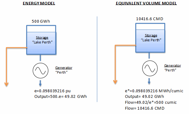Figure 7: Equivalent volume model for storage "Lake Perth"

Then, in order to produce the same amount of electrical energy out of 'Pert', the total water flow through the generator must be 10416.6 CMD (see Figure 2). Same applies to other storages upstream.

Table 11: Storage Input for Hydro-Cascade Volume Model

Property	Max Volume CMD	Initial Volume CMD
Lake Adelaide	120833.3	-
Lake Brisbane	191666.7	-
Lake Melbourne	41666.7	20833.3
Lake Perth	20833.3	10416.7

The total potential energy from each of the two (only) natural incomings will be used by all three generators downstream. Given that the efficiencies sum the unity, as shown in Table Y, the conversion is straightforward:

inflow [MW]=inflow[cumec]

The table presented next, shows the equivalent volume model taking the above assumption.

Table 12: Natural Inflows Used for the Energy and Volume Module

Month	Natural Inflows GWh	GMD
Jan	1996.98	287.93
Feb	14607.1	350.57
Mar	15470.68	371.3
Apr	15806.24	379.53
May	13436.16	322.47
Jun	7133.39	171.2
Jul	615.77	14.78
Aug	2058.33	49.4
Sep	12913.33	309.92
Oct	16920.51	406.09
Nov	19011.48	456.28
Dec	13950.78	334.82

Note that total volume of the natural inflows is usually reported in CMD (metric system) as follows:

inflow [CMD]=inflow[cumec]*1000*(3600/86400)

As it was expected, the results are equivalent as in the energy model.

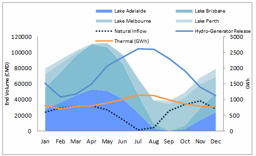Figure 8: Hydro-thermal co ordination results for Case 9. Volume model results.

There are several reasons why the volume (and level) model is more accurate and adequate over the energy model.

• The Volume and Level models are based on the physical relationships of hydrological objects. Therefore, they are in nature easier to understand.
• Preparation of cases in the energy model is usually harder because potential energy availability needs to be pre-computed considering every generator downstream.
• Statistic data and measures are usually given in volume of water.
• The most important among several drawbacks of the potential energy model is that when there are several ways to which the water can run downstream, there is not an obvious way to determine in advanced the amount of energy that is going to flow through each of the alternative spillways.

7. Hydro Visualization Tools

PLEXOS 6 implements geographical visualization tools for Hydro and Transmission systems. On the main PLEXOS menu, the visualization button will launch the configuration dialog as it is shown in figure

Geospatial data in KML format can be read and displayed in Google Earth. Screenshot of the NZ hydro system in Figure 10: NZ hydro and transmission system in Google Earth visualization.

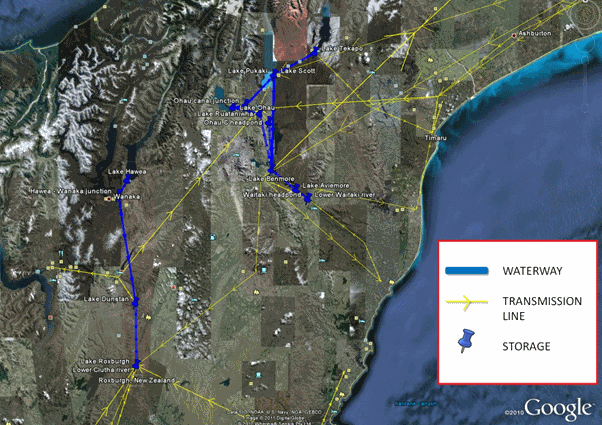Figure 9: NZ hydro and transmission system in Google Earth visualization

PLEXOS also supports export of the transmission and hydro systems to Geographic Markup Layout (GML) format which can be read by a number of commercial and freeware viewers such as Cytoscape.

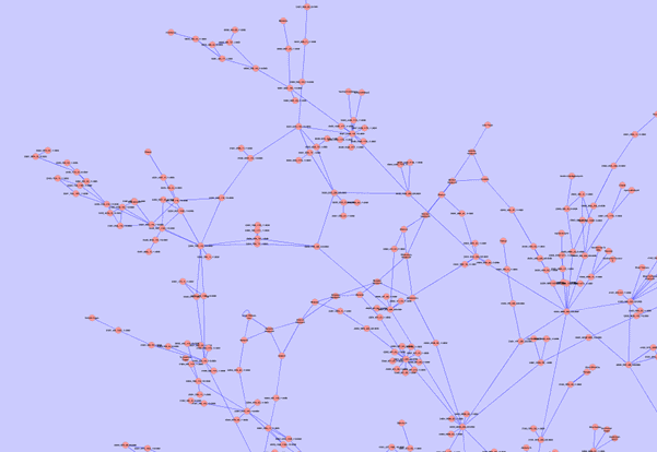Figure 10: NZ transmission system visualization in Cytoscape