Gas Modelling
Contents
1. Introduction
PLEXOS is an Integrated Energy Model, bringing together Electric and Gas Models. The simulator provides these classes for the Gas Model:
| Class | Description |
|---|---|
| Gas Basin | Summary class to contain a collection of gas producing fields |
| Gas Capacity Release Offer | The release of available pipeline or storage capacity to another party. |
| Gas Contract | Contract for producing gas |
| Gas Demand | Demand for gas |
| Gas DSM Program | Demand side management programs |
| Gas Field | Field from which gas is extracted |
| Gas Node | Connection point in gas network |
| Gas Pipeline | Pipeline for transporting gas |
| Gas Plant | Gas processing plant for converting raw natural gas to pipeline quality |
| Gas Storage | Storage where gas can be injected and extracted |
| Gas Transport | Gas shipment |
| Gas Zone | Collection of gas nodes |
The Gas Model provides the capability to model the costs and constraints of gas delivery from its source fields via a network of pipelines, processing plants/facilities, through storages and on to meet demands including those in the Electric Model. The Gas Model integrates with LT Plan to calculate optimal investment decisions for both gas and electric assets.
Note that this integrated Gas/Electric Model is not intended to perform the function of a gas pipeline flow model. Rather, it uses a simple transportation algorithm to model gas flows.
2. Gas Model
2.1. Network Definition
The Gas Model is composed of objects from the classes listed above. These connect together as shown in Figure 1.
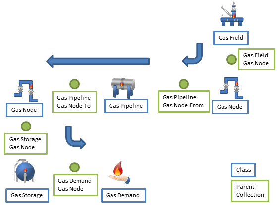 Figure 1: Gas Model
Your Gas Model may include any number of these objects in any configuration.
2.2 Units of Data
The Gas Model tracks flows of gas through the network from its source in Gas Field and/or Gas Storage objects to consumption by Gas Demand and/or Generator objects.
The unit of gas volume and flow varies depending on the Units of Data setting:
- Terajoule (TJ) for metric system
- Million cubic feet (MMcf) for imperial U.S. system
Units of gas pricing, such as the Gas Field Production Cost
- $/Gigajoule ($/GJ) for metric
- $/million British Thermal Unit ($/MMBTU) for Imperial U.S.
Input quantities such as Gas Demand Demand are expressed as quantities consistent with the given Horizon Periods per Day. For example if Periods per Day = 48 (half-hourly) and you define Gas Demand Demand = 100 TJ (or MMcf) then this amount will be demanded in that half hour. If you change Periods per Day to 24 (hourly) then the 100 will be demanded in one hour. This is in contrast to the Electric Model where many input properties are (time invariant) rates such as megawatt.
Unit in Gas objects allows you to override the default setting and select between a wide range of in-built units (listed below) or to leave the Gas object unit-less and it will default based upon the setting (Metric or Imperial). This allows the modeling of systems with different units, such as allowing a Gas Field data to be entered in GJ while in an Imperial system using MMBTU as the default Gas Unit. The user-interface will display the selected Unit in the "Units" column of the property grid.
The following units are available:
|
Commodity Unit |
Type |
Name |
Base Units/Metric |
|
kJ |
Energy |
kilojoule |
1E+3⋅kg·m2·s−2 |
|
MJ |
Energy |
megajoule |
1E+6⋅kg·m2·s−2 |
|
GJ |
Energy |
gigajoule |
1E+9⋅kg·m2·s−2 |
|
TJ |
Energy |
terrajoule |
1E+12⋅kg·m2·s−2 |
|
PJ |
Energy |
petajoule |
1E+15⋅kg·m2·s−2 |
|
EJ |
Energy |
exajoule |
1E+18⋅kg·m2·s−2 |
|
MMBTU |
Energy |
million BTU |
1.055056E+9·J |
|
BBTU |
Energy |
billion BTU |
1.055056E+12·J |
|
Dth |
Energy |
dekatherm |
1.055056E+9·J |
|
MDT |
Energy |
million dekatherms |
1.055056E+15·J |
|
MCF |
Volume |
thousand cubic feet |
1.095148E+9·J |
|
MMCF |
Volume |
million cubic feet |
1.095148E+12·J |
|
TOE |
Energy |
tonne equivalent of oil |
4.1868E+10⋅kg·m2·s−2 |
|
kTOE |
Energy |
thousand TOE |
4.1868E+13⋅kg·m2·s−2 |
|
MTOE |
Energy |
million TOE |
4.1868E+16⋅kg·m2·s−2 |
|
bbl |
Volume |
42 gallon barrel |
158.987·L (6.12E+9·J) |
2.3. Storage
The classes Gas Field, Gas Storage and Gas Pipeline all act as storage for gas. Gas Field is the simplest case where you set the Initial Volumeand the Production Cost.
For Gas Storage the "working capacity" is between the Min Volume and Max Volume and there is Injection Charge and Withdrawal Charge
The Gas Pipeline class models "line pack" as gas stored in the pipelines. The bounds on line pack are Min Volume and Max Volume and charges such as Flow Charge can be defined.
The Gas Plant class models the gas processing capacity of gas plants to convert raw gas into saleable pipeline quality gas. The processing capacity is limited by the Min Production and Max Production, and the cost of processing is defined by the Processing Charge.
These storage elements act similarly to hydro Storage objects in the electric model:
- How end-of-horizon gas volumes are constrained or valued is controlled by the End Effects Method property on those classes.
- Their mid-term sequence of end volume and/or shadow price can be passed for LT Plan or MT Schedule to ST Schedule according to the Decomposition Method property on those classes.
With these features you are able to optimize the medium to long term usage of gas fields and storage while still modelling fine detail in ST Schedule.
3. Electric Model Integration
The Gas and Electric Models integrate at the Gas Node. A Generator can be attached to a Gas Node via the Gas Node and Fuel Gas Nodes memberships. Defining both these memberships instructs the simulator that the Generator is physically supplied with Fuel from the Gas Node and it will demand gas according to its Heat Rate and Generation. Thus connected Generator objects must have memberships to one or more Fuel objects. This is illustrated in Figure 2 which shows Generator objects connected to the gas network, and also associated with Fuel objects, some of which are delivered via the gas network, others that are independent e.g. to model multi-fueled generators that can burn fuels other than gas.
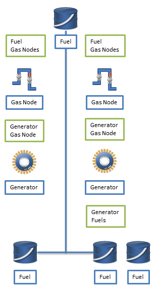 Figure 2: Integrated Gas Electric Model
You may use the Fuel objects act as the financial side of gas delivery i.e. the Gas Model might include only constraints on the gas delivery (e.g. Gas Pipeline limits) and transport charges, whereas the Electric Model's Fuel (and optionally Fuel Contract) objects define the cost of gas. Alternatively all costs can be defined in the Gas Model. It is noted that the two cost methods should not be used at the same time.
4. Expansion Planning
The following classes can be built/retired automatically by the LT Plan
To define an expansion candidate set the Max Units Built property to unity and the Units property to zero. You can then define the Build Cost and other parameters.
The Gas and Electric Models are co-optimized in LT Plan meaning that optimal decisions are made considering the total cost of the two system combined. Thus it is possible to find the optimal combination of Gas and Electric asset investments/retirements over the horizon.
The optimal expansion decisions from LT Plan are automatically passed to subsequent simulation phases including the expansion of the Gas System.