Storage Optimization
Contents
This article describes deterministic and Monte Carlo modelling of hydro reservoirs and the coordination of storage between MT Schedule and ST Schedule. Refer to Multi-stage Stochastic Optimization regarding multi-stage stochastic optimization of storage.
1. Introduction
Hydro networks commonly contain both short-term and long-term storage:
- Short-term storage like pumped storage, regulation tank/canal and small head pond storage can set their release policy within a day or week long window.
- Long-term storage optimize their release policy over a window of several months or years.
The simulation should be set up with consideration to these questions:
- Is the optimization step long enough that it can 'see' the future value of long-term storage e.g. in displacing future thermal or shortage costs?
- Is the optimization resolution fine enough to capture the short-term value of storage e.g. in balancing short-term fluctuations in load and/or renewable generation?
It is generally impractical to run the simulation with both sufficient resolution and a long enough optimization window, thus the simulation horizon is usually divided into a number of 'steps'. Here we describe how short and long-term storage are managed across multi-step and multi-phase simulations.
2. Short-term Storage
2.1. Step Length and End Effects
ST Schedule, configured correctly, can optimize releases for short-term storage. The resolution and optimization window are controlled by Horizon settings. The size of the step is controlled by Horizon Chrono Step Type and Chrono At a Time.
The following table provides some examples. It describes how a Horizon of one year would be simulated given the particular settings:
| Chrono Step Type | Chrono At a Time | Step Size | Number of Steps | Notes |
|---|---|---|---|---|
| "Day" | 1 | 1 day | 365 | 365 for leap years |
| "Day" | 7 | 1 week | 52 | Only 364 days simulated |
| "Week" | 1 | 1 week | 52 | Only 364 days simulated |
If the simulation horizon is a discrete number of weeks, e.g. 52 weeks, then a weekly step type is ideal, but for modelling a true calendar year, the day step type is more practical. The potential problem with a day step type is that the optimization cannot 'see' the future value of storage. A week step type might also be impractical in terms of simulation size and runtime, moreover it is blind to the future value of storage beyond the end of the week and thus, in the absence of constraints, might use all the available water before the end of the week. This issue is referred to as "end effects".
The simulator provides two features to address these issues:
2.2. Look-ahead
Look-ahead improves the optimization by allowing each step to 'see' further into the future. For very short-term storage adding a day of look-ahead may be sufficient, but additional look-ahead may be required for larger storage. Look-ahead is configurable with a lower resolution than the base horizon, thus the advantage of greater foresight can be obtained without adding significant computing overhead.
The following table provides examples for the set up of look-ahead:
| Periods per Day | Chrono Step Type | Chrono At a Time | Look-ahead Type | Look-ahead At a Time | Look-ahead Periods per Day | Step Size | Notes |
|---|---|---|---|---|---|---|---|
| 24 | "Day" | 1 | "Day | 1 | 24 | 2 days | 1 day's solution is retained, 1 day lookahead is discarded each step |
| 24 | "Day" | 1 | "Day" | 6 | 8 | 7 days | Hourly resolution with look-ahead 3-hourly. 1 day's solution is retained, 6 days of lookahead is discarded each step |
| 144 | "Hour" | 6 | "Hour" | 18 | 24 | 1 day | 5-minute resolution with look-ahead at hourly resolution. 6-hour's retained, 18 hours discarded each step |
Note that the total Horizon length must accommodate the look-ahead e.g. if you add a day of look-ahead your horizon should include one extra day. If your Data File objects do not contain sufficient data, the simulator will pad out the additional days matching data by period of day.
2.3. End Effects Method
Look-ahead alone might not trigger multi-day storage and pumped storage to hold sufficient water for future days/weeks in all circumstances. A stricter regime is to cycle the storage level back to its starting point on a regular basis. The simulator automatically implements this 'recycle' policy when it detects that no other constraints are being used to manage the storage (such as Storage Target or Constraint End Volume Coefficient).
The automatic recycle constraint ensures that the storage returns to its initial volume/level at the same period each day e.g. midnight-to-midnight. This automatic setting can be over-ridden with the Storage End Effects Method property.
If the simulation step is longer than one day, the recycle point is the last matching hour of each day, e.g. last midnight, in the step. If the simulation step excluding look-ahead is shorter than one day, it is important to add look-ahead so that the step is a day in duration in total, or the recycle constraint will be inappropriate. In high-resolution simulations, e.g. 5-minute resolution, running a lower resolution e.g. hourly look-ahead so that the total step length is at least a day is very important for storage optimization.
Note: An option is available if you prefer to ignore the look-ahead periods. See Hidden parameters for more information.
2.4. Interleaved Simulations
Interleaved simulations involve two (or more) Model objects executing together with the steps of execution interleaved and data being passed between the models at each step. The interleaved relationship is established through the Model Interleaved membership.
Interleaved simulations automatically pass the Storage End Volume from the interleaved model back to Storage Initial Volume in the master model. This means you can perform very high resolution simulations in the interleaved model while maintaining a longer optimization horizon in the master model e.g. for unit commitment or hydro optimization.
In conclusion, short-term storage is optimized by a correctly configured ST Schedule.
3. Long-term Storage
Long-term storage presents similar issues to short-term with the additional complication that ST Schedule is generally too high resolution (and too computationally expensive) to run in steps long enough to fully optimize these storage. The solution is to optimize long-term storage in the MT Schedule phase of the simulation. By default, MT Schedule runs in one-year steps, and this can be further extended with the MT Schedule At a Time attribute to any length up to the Horizon duration. This optimization has a long enough 'window' to optimize release policy, although you will still need to decide the end storage policy with the Storage End Effects Method property or storage bounds, targets or constraints.
To run such a long simulation step MT Schedule reduces the resolution of the simulation. MT Schedule is highly configurable and can run very high resolution, but it defaults to just 12 time blocks per week. This provides good performance over long horizons, but it sacrifices accuracy in the short-term. This implies that short-term storage, batteries and pumped storage will not be fully optimized. The solution is to combine MT Schedule and ST Schedule in a single optimization run, with long-term storage optimized by MT Schedule and long-term by ST Schedule.
3.1. MT Schedule and ST Schedule
As described in the Hydro Thermal Coordination article, MT Schedule and ST Schedule automatically manage long-term storage.
A policy should be defined for long-term storage e.g. by setting the Storage End Effect Method = "Recycle" or defining Storage Target. Then configure MT Schedule so that the simulation steps span a period sufficient to see the target period or the recycle period e.g. recycling will default to each year because MT Schedule runs annual steps by default.
After MT Schedule completes it automatically passes information to ST Schedule. By default Storage targets are created for each step of ST Schedule e.g. each day or week step gets a unique storage target that follows the Storage End Volume from MT Schedule.
The target method of decomposition (coordinating the simulation phases) is generally best, but the Storage Decomposition Method property allows for different methods such as price-based decomposition.
3.2. Resolution Considerations
The Chronology and resolution of MT Schedule and ST Schedule. If MT Schedule Chronology = "Partial" (the default) it uses load duration curves (LDC) to compress the chronology and there is no "tracking" of storage inside each LDC e.g. if you use a monthly LDC, then the storage is only "balanced" every month i.e. inside the month the storage is not calculated and so storage bounds are not enforced intra-month, only at each month boundary.
If you then run ST Schedule with daily steps, it can be somewhat difficult for MT Schedule to provide correct storage targets or price signals to ST Schedule. If the storage is large, and unlikely to hit more than one bound in a month, this potential compromise can be acceptable, and the simulator attempts to provide the best possible coordination signals to ST Schedule no matter what LDC settings are used in MT Schedule.
Although MT Schedule only provides storage end volume figures at LDC boundaries, the release and inflows decisions occur each LDC block, and thus every original hour in the horizon can be mapped to a releases/inflow pair at the storage. Thus a chronology for the storage can be synthesized. Such a synthesized chronology is illustrated in Figure 5.
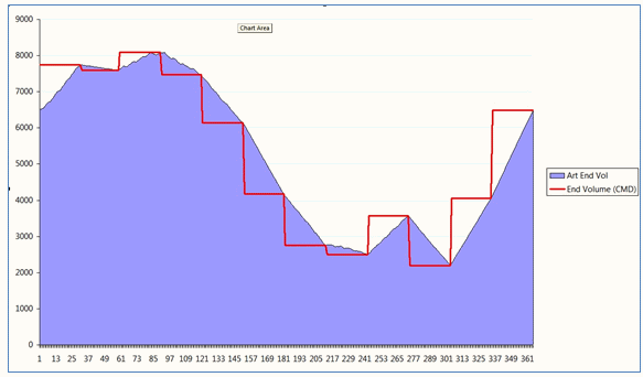 Figure 5: Synthesized End Volume Solution from MT.
The red line in Figure 5 shows the Storage End Volume results from MT Schedule as one-value-per-month. The continuous upper envelope of the area in the same figure shows the synthesized chronology based on the LDC block-by-block release/inflow results mapped back to hours. This chronology map can provide a reasonable trajectory for ST Schedule to follow down even to an hourly resolution (though in this case a daily ST Schedule step is as fine a resolution as seem sensible).
These considerations still apply somewhat when MT Schedule Chronology = "Fitted" or "Sampled" though to a lesser degree since in those schemes chronology is preserved but resolution is reduced, so this effect is only apparent when ST Schedule has a sub-hourly time step.