Nodal Area Interchange Logic

An Aggregate Area may be represented as a study area (Solution Method = OPF) or an external area (Solution Method <> OPF). Study areas are the aggregate areas which represent the market or system that is of immediate modeling interest. It generally consists of some subset of a larger interconnected system. External areas are those aggregate areas which are outside study area but, as part of the larger interconnected system, are expected to materially impact flows and dispatch patterns within the study area.

You can model interchange constraints between study areas or between study and external areas. Moreover, several options exist for the representation of external areas, again with the purpose of capturing interchange between study and external areas without modeling the full network of external areas. In the discussion below we describe interchange handling in Aurora, beginning with study aggregate area constraints and then with the representation of, and constraint handling for, external areas.

Study Area Constraints

The model allows the user to specify bulk transfers between study areas via the Net Exports column, which can take different values, including (1) positive and negative numeric values, (2) a null (or blank) value.

Positive or negative numeric values - When a numeric value is entered in the Net Exports column for an Aggregate Area, either directly with a number or indirectly via a time series reference, the model imposes a constraint on the same aggregate area, such that for each hour:

Generation = Demand + Net Exports

In other words, aggregate area generation must exceed demand by the amount of the assumed net export. A positive net export value then indicates an hourly outflow while a negative value indicates an hourly inflow. A 0 (i.e., zero value) forces a balance between generation and demand in the Aggregate Area.

When non-null values are specified for one or more study areas, and the values do not exactly cancel each other out across all external areas, at least one study area must have Net Exports set to null or at least one external area must have a value of Econ in order for the excess to be absorbed. In other words, the entire footprint of areas, both system and external, is a closed system.

Null values - The model will put into a single aggregate area constraint the study areas which have null (i.e., blank) Net Export values, such that the sum of the Net Exports across the all of the study areas is zero (this is a requirement of the OPF, namely that generation equals demand).

External Aggregate Area Representation

When an aggregate area is represented as an external area (Solution Method <> OPF, Composite Buses = True), the external area is composed of a composite generator bus and a composite demand bus. Transmission elements within an external area are not represented, but transmission elements between an external area and a study area or between two external areas are represented. Weighted average shift factors distribute the flows to and from the composite generators and composite demand across the inter-area transmission elements.

Demand for an external area is handled similarly to that of a study area. The external area demand is the hourly zonal demand aggregated according to the relationships specified in the AURORA Zone Map table. Since the external area has demand at a single composite bus, there is no further handling of demand beyond the aggregate area. (For study areas, demand is in turn distributed from the aggregate area to the bus level via the nodal area.)

External area generation is handled using a composite generator with multiple segments based upon the corresponding zonal resources. The composite generator will be dispatched so as to respect the aggregate area constraints that are specified.

External Area Constraints

As with study areas, constraints can be imposed on external areas through the Net Exports column. The three possibilities are (1) a Ref or null value,(2) an Econ value or (3) a positive or negative numeric value.

Ref or Null values - When a Ref or null (i.e., blank) value is specified in the Net Exports column, the model dispatches the composite generator at the dispatch levels from the underlying (solved) load flow case.

An Econ value - When an Econ value is entered, the model represents the composite generator with a dispatch cost structure which reflects the merit-order resource stack for the external area. By default, the model creates twenty equal production cost segments. As with any dispatchable generator, the OPF determines the optimal dispatch of the composite generator, and therefore the interchange to and from the external area.

Positive or negative numeric values - This works in the same manner as for study areas. Use the Apply aggregate area interchange constraints option in the nodal Solution Settings folder of Simulation Options to apply this logic. Use of Econ and Ref settings for external areas is possible without the switch turned on since neither of these two settings creates constraints beyond the system supply and demand constraint.

Multiple Island Handling with External Areas

When an aggregate area is represented as an external area (Solution Method <> OPF, Composite Buses = True), it is possible that it can break the transmission between the study (or OPF) areas. However, Aurora allows multiple islands to exist within a case. As the diagram below shows, the external areas cut the system into two islands, West and SE. Internal congestion within the external areas will not be modeled.

Simulation Logic

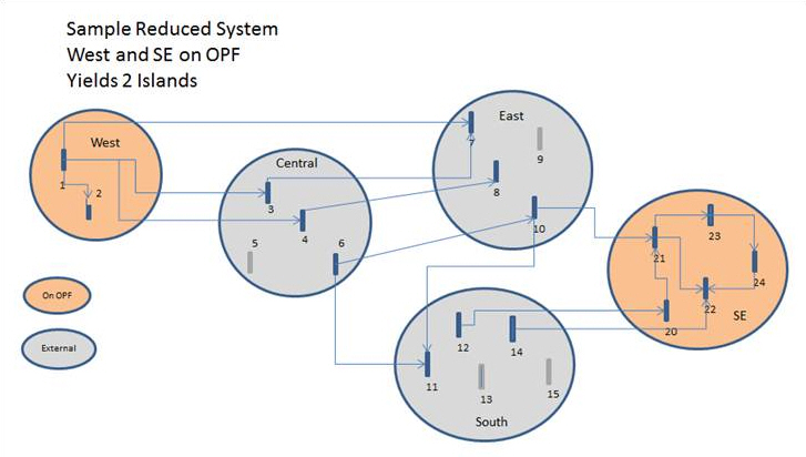
Nodal External Area Interchange Logic