Setting Up the Multi-stage Stochastic Optimization Feature
Contents
- Introduction
- Model Set Up
- Sampling
- Rolling Horizon
- End of Horizon Water Values
- Non-anticipativity Constraints
- Future Cost Function
- References
This article describes multi-stage stochastic optimization of hydro storage.
Prerequisites:
1. Introduction
This article describes multi-stage stochastic optimization by the Rolling Horizon solution method. Rolling Horizon is a robust and efficient solution method for multi-stage optimization. By solving in a single pass without the need for repeated forward and backward iterations, it guarantees convergence and optimality. The method naturally handles complexities such as integer decision variables, non-convex elements, negative price outcomes etc, making it superior to 'traditional' stochastic dual dynamic programming.
Because of its ability to optimize integer decisions, Rolling Horizon is the default stochastic algorithm for LT Plan. For MT Schedule you can choose between Rolling Horizon and SDDP, depending on your needs.
2. Model Set Up
This section details the steps required and recommended to set up multi-stage stochastic simulation and solve via the Rolling Horizon method. It is also a guide to converting an existing deterministic hydro model to a multi-stage stochastic model.
Rolling Horizon for multi-stage stochastic hydro optimization is available in LT Plan and MT Schedule. The method is automatically triggered when LT Plan Stochastic Method or MT Schedule Stochastic Method = "Stochastic" and there is a multi-stage scenario tree defined in any Global object. However the set up of the tree and supporting input data and simulation settings is somewhat complex. Here we address each aspect of the set up in detail.
2.1. Horizon and Simulation Phases
Rolling Horizon always solves the Horizon in one 'step' i.e. a window of time spanning the entire horizon, but it does so using multiple iterations or 'rolls'. The Horizon should be configured to a single step by setting the same period type and same number of periods in MT Schedule:
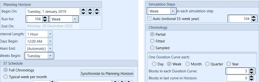 Figure 1: Example Horizon Settings
In this example, the entire 104 week horizon will be run in one step of MT schedule.
When LT Plan is the first simulation phase, use the default step size settings to optimize the entire planning horizon in one 'step'. While the one 'step' setting and Stochastic Method = "Stochastic" should apply only to the rolling horizon phase, the following phases need to run "Monte Carlo" or "Deterministic" within any number of steps.
2.2. The Scenario Tree
The scenario tree is the most important input to the multi-stage stochastic optimization. The rolling horizon solution method expects the tree to have a combination of full branches and hanging branches:
- Full branches are regular scenarios that span the simulation horizon and are reported to the solution file.
- Hanging branches are supplementary scenarios that exist only from a given stage (week/month) and out to the end of the horizon. These branches provide detail to the scenario tree but are discarded from the solution file.
Thus in a rolling horizon model with hanging branches there are more total scenarios in the simulation than scenarios written to the output. The number of samples defined by Stochastic Risk Sample Count equals the total of full branches plus hanging branches. The relationship between total samples, full branches and hanging branches is as follows:
Risk Sample Count = Full Branch Count + Full Branch Count × (Stage Count - 1) × Hanging Branches (per Stage)
2.2.1. Basic Concepts
In the following figure, a 4-stage tree is illustrated with 3 full branches and 2 hanging branches per stage.
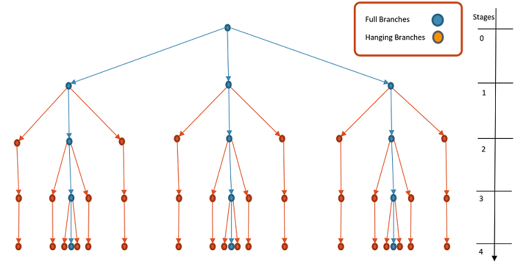
With some basic concepts defined as:
- Stages: Time when new infor is revealed
- Root Node: Current state at stage 0
- Node: A possible state associated with a set of data: demand, inflow, etc...
- Branches: Scenarios for next stage
- Scenario: A path from root to a leaf
2.2.2. Scenario Tree Creation Wizard
A scenario tree can be defined in a Global Object by setting related properties: Tree Stage Count, Tree Period Type, Tree Stages Position, Tree Stages Leaves and Tree Stages Hanging Branches. The Scenario Tree Wizard can be used to easily define a tree as desired. This is accessed by right-clicking the Global collection and selecting Scenario Tree Wizard as follows:
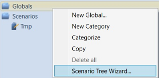 Figure 2: Scenario Tree Wizard Settings
The first page of the wizard lists the Horizon objects found in the database, and automatically suggests sensible values for the period type and stage count for the scenario tree. The second page of the wizard provides a view of the resulting tree with specified number of full branches and hanging branches. The data created by the wizard can be tagged with a particular scenario from the drop-down list.
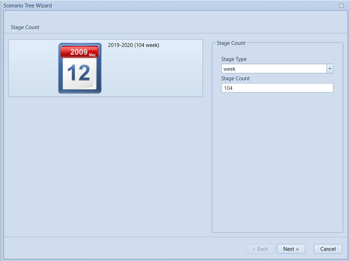 Figure 3: Scenario Tree Wizard page 1
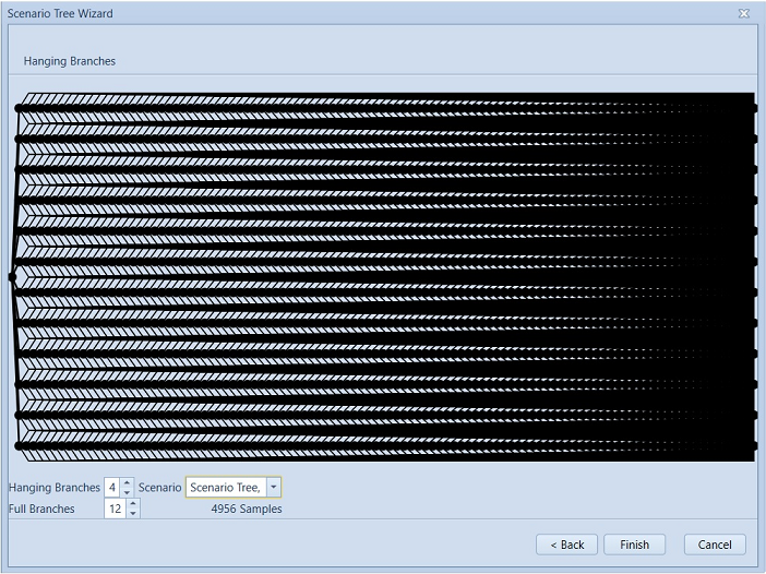 Figure 4: Scenario Tree Wizard page 2
This then automatically creates a Global object and related properties to represent the tree within the simulation.
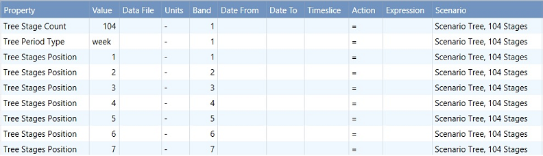 Figure 5: Tree properties created using Scenario Tree Wizard
The number of samples in scenario tree should match Risk Sample Count. The wizard in Figure 4 also displays the resulting number of samples, which is calculated by the formula for Risk Sample Count stated above. This should be input as the same number for variable sample draws in Stochastic Setting as in Figure 6, since the scenario tree has 4956 samples with 12 full branches, 4 hanging branches and 104 stages defined.
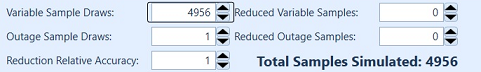 Figure 6: Sample numbers in Stochastic Setting
Otherwise, user could just leave Risk Sample Count as 1 and the total samples for scenario tree: 4956 will be automatically computed from the input and printed to the log file.
2.2.3. Scenario Tree Creation (Simplified settings)
Because it is most common to define trees with the same number of leaves and hanging branches at each stage and with evenly spaced stages, we have allowed the input of only band 1 for the Tree Stages Leaves and Tree Stages Hanging Branches inputs and the complete omission of Tree Stages Position. The following simplified settings creates the same scenario tree as what the Wizard does in the above example:
| Property | Value | Data File | Units | Band |
|---|---|---|---|---|
| Tree Period Type | Week | - | 1 | |
| Tree Stages Leaves | 12 | - | 1 | |
| Tree Stages Hanging Branches | 4 | - | 1 |
In case where the user needs to define a tree with unevenly spaced stages, Tree Stages Position or Tree Stages Position Incr can be used to specify them by bands. Please note that from PLEXOS 9, the input Tree Stages Count has been removed, which will be implied by the period count of the horizon (i.e. 104 week for this simplified case) or Tree Stages Position and Tree Period Type properties.
2.3. Hanging Branches Block Count
With the LDC settings in Figure 1, 5 blocks per LDC will be formulated for full branches. To consider the performance, by default, only one block per LDC will be modelled for hanging branches. The property Hanging Branches Block Count could be used to achieve faster performance, by limiting the time periods modelled after the hanging branch begins. Examples could be found in Hanging Branches Block Count.
3. Sampling
The aim of stochastic hydro optimization is to determine under uncertain situations, what the optimal solution is for the End Volume of Storages and dispatch of Generators. The uncertainty comes from unpredictable future inflows into storages, which is modelled using the Variables class in PLEXOS. Once the inflow variables are defined and historical data is provided, two sampling methods, historical sampling or PARMA sampling, could be used to populate the scenario tree, i.e. determining the sample values for each scenario. These two methods are quite different in terms of configuration and implementation.
3.1. Historical Sampling
Historical sampling assumes that the future repeats itself on full branches, and that the information in different years represents the uncertainty on hanging branches. Figure 7-8 is an illustration of how historical data is mapped into full branches and hanging branches.
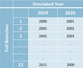 Figure 7: Mapping to full branches
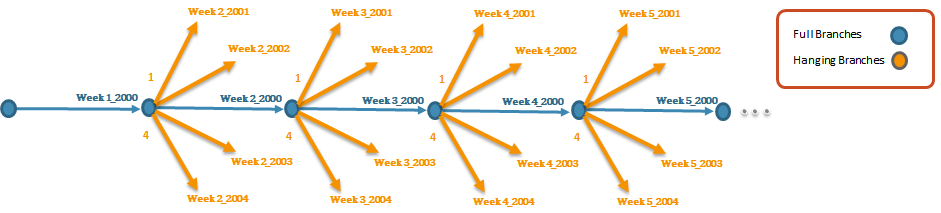 Figure 8: Mapping to hanging branches
This section details the steps required to set up and achieve the above mapping.
Historical Sampling will be invoked when the Data file attribute Historical Sampling is enabled. The input Data file should include historical data for the tagged Variable and should have the Historical Period Type set as week or month.
| Historical Sampling (Yes/No) | Historical Year From | Historical Year To | Historical Year Start | Historical Period Type |
|---|---|---|---|---|
| Yes | 2000 | 2011 | 2000 | Week |
| Collection | Parent Object | Child Object | Property | Value | Data File | Units | Band |
|---|---|---|---|---|---|---|---|
| Data Files | System | Water | Filename | 0 | Water.csv | - | 1 |
| Variables | System | Inflow | Profile Week | 0 | Water | - | 1 |
By default, the sampling range starts from the first year and end to the last year of the historical data, with specific week/month matched to horizon starting week/month. In the example of Figure 7-8, we have 12 years' weekly data provided via data file Water.csv ranging from 2000 to 2011, and horizon setting 104 weeks from 2019-2020 as shown in Figure 1. Please note that in the case the historical data file has a YEAR/WEEK format, an assumption has been made that the first week always contains the first day (January 1st) of the calender year, so the specific date for the day each week begins with can be worked out for the data to associate with. Sampling will be then based on those dates and values. It will try to match the days of the week as closely as possible so it can choose to move forward or back one week in order to get the best match to the weekday of January 1st.
Historical Year From, Historical Year To, Historical Year Start can be used to set the range and the start year for sampling. Sampling then will be starting at Historical Year Start inside the sampling range and loop back to Historical Year From after Historical Year To. When multiple full branches are defined, it chooses consecutive years by default as the first year for each full branch staring from the Historical Year Start, eg. year 2000 for the 1st full branch, 2001 for the 2nd, 2002 for the 3rd, and so on.. From versions above PLEXOS 9.0 BETA 2.0, user has the option to select alternatives by defining Full Branches Historical Year Start for each full branch in one band.
It could also be specified from which years hanging branches will be starting by using Hanging Branches Historical Year Start as in the following example:
| Property | Value | Data File | Units | Band |
|---|---|---|---|---|
| Hanging Branches Historical Year Start | 2001 | - | 1 | |
| Hanging Branches Historical Year Start | 2002 | - | 2 | |
| Hanging Branches Historical Year Start | 2003 | - | 3 | |
| Hanging Branches Historical Year Start | 2004 | - | 4 |
When the historical data spans a large amount of years, the start years selection for hanging branches could be a problem. By turning on the Hanging Branches Sample Reduction setting to be True, users don't need to specify the historical start years which will be automatically determined by scenario reduction algorithm and printed out to the log file.
Please note that if a hanging branch is selected as the same as one of the full branches, the hanging branch start year will be swapped with an alternative year in the historical dataset to ensure unique samples.
The "User" Sampling Method should be selected for historical sampling.
| Property | Value | Data File | Units | Band |
|---|---|---|---|---|
| Sampling Method | User | - | 1 |
While Inflow data for multiple storages could share a single data file, multiple variables should be defined with each variable standing for inflow for each single storage.
3.1.1. Sampling with higher resolution data
Historical sampling also allows a profile to be sampled on a week-to-week basis but have underlying data with a higher resolution. This can be achieved by selecting a variable period type that matches the data resolution, e.g. Profile Day for daily inflows and Profile for hourly wind.
| Collection | Parent Object | Child Object | Property | Value | Data File | Units | Band |
|---|---|---|---|---|---|---|---|
| Variables | System | Inflow | Profile Day | 0 | Inflows | - | 1 |
| Variables | System | Wind | Profile | 0 | Wind | - | 1 |
3.1.2. Sampling with multi-band forecast data
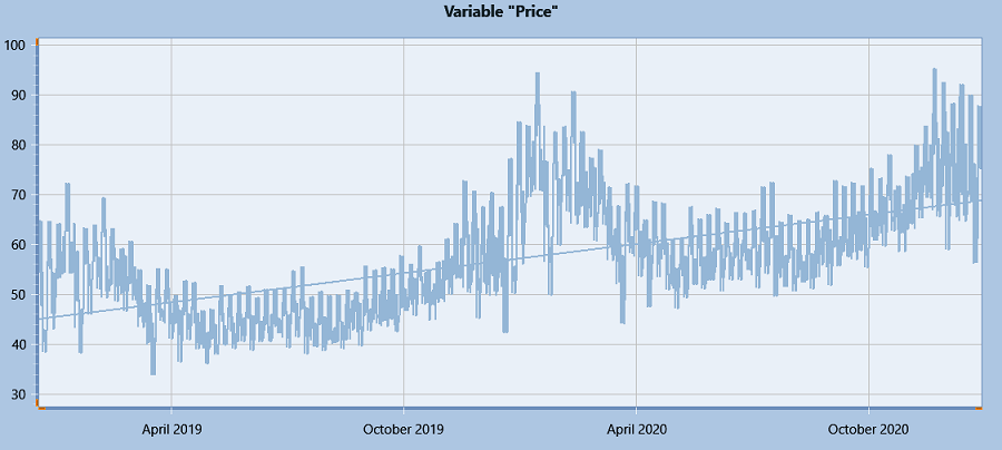
For certain profiles like external market prices, the data could be weather-dependent similarly as inflows and wind, but also have trends over the simulation horizon. It requires combining historical sampling with a future series of data to deal with two correlations: correlation between historical year and market price AND correlation between future year and the price. For example, market prices could be higher in a historical year when inflows are lower, but generally increasing over time. This can be done by sampling a profile with an input format of Year, Month, Day, Period for the planning horizon (2019 -) and multiple Bands corresponding to the index of the historical year (Band 1 for 2000, Band 2 for 2001, etc.), e.g.
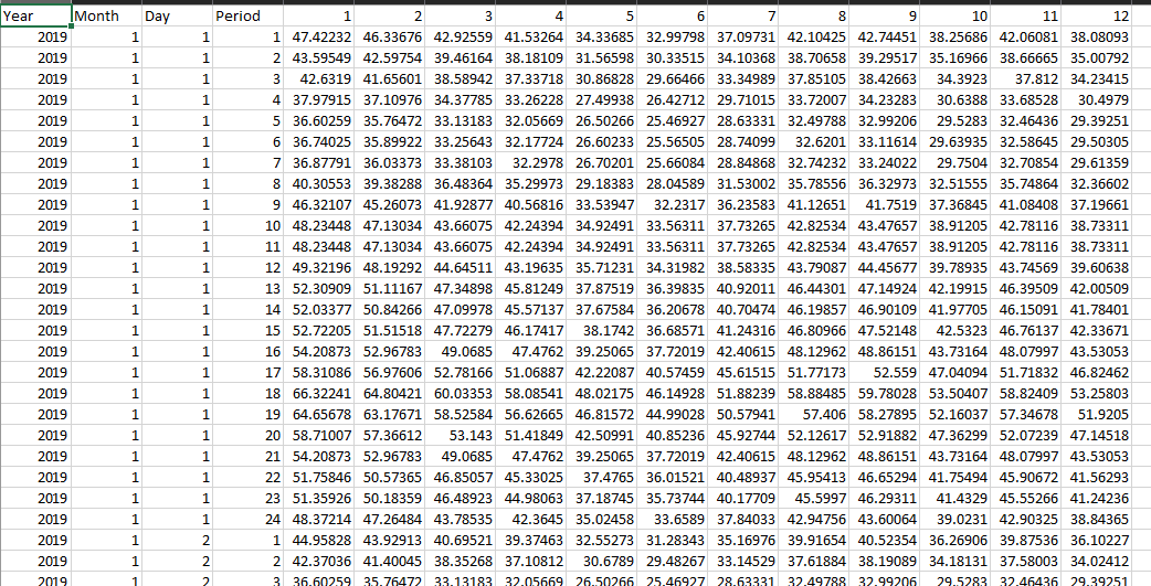
This file will be processed with historical sampling, and the outcome of the first full branch (hourly resolution) - in this case it selected Band 4 of the file shows the upgrade escalation in market prices over the horizon as desired.
Please note that when historical sampling is required for a profile other than storage natural inflow, such as Wind, Market Price, etc., the option Rolling Horizon With Other Variables needs to be set as True.
3.2. PARMA Sampling
The Historical sampling method well preserves the correlation between different hydro basins and is very fast as no randomness involved. However, one disadvantage of the method is that not looking at the past when branching can lead to jumps between dry and wet inflows between stages. Furthermore, the number of full branches is limited to the total years of historical data (i.e. 12 for this example). PARMA sampling is an option to overcome these obstacles.
PARMA sampling automatically fits the historical data with time series models for each inflow variable, and considers spatial correlations between them. SARIMA (Seasonal Autoregressive integrated moving average) and PAR (Periodic Autoregressive) are a class of time series models frequently used for seasonal or periodic series forecasting, which are able to capture the temporal correlations between past and future. Detailed model descriptions and parameter estimation methods can be found in the reference paper [1],[2]. With fitted parameters, the sample values will then be simulated by the PARMA dynamics with random normal errors.
PARMA sampling will be enabled via the option PARMA Model Type with 0 for using SARIMA model, 1 for PAR model and -1 for None which means turning off PARMA sampling.
| Historical Sampling (YES/NO) |
|---|
| YES |
Note that there is one setting that will be different from Historical sampling (using Historical variables) when using PARMA sampling (using PARMA variables), which is the Sampling Method. It should always be "Auto" for PARMA variables but "User" for Historical variables.
| Property | Value | Data File | Units | Band |
|---|---|---|---|---|
| Sampling Method | Auto | - | - | 1 |
There is an option to print out the estimated parameters to a csv file diagnostic for each inflow:
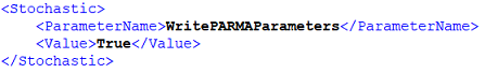
Samples generated by either sampling method could be written out by switching on the diagnostic option "Historical Sampling" in the Diagnostic class. Advanced settings for PARMA include methodology selection for simulating the scenario tree using Brazil Scenario Tree and options to combine Historical sampling for full branches using Historical Full Branches.
4. Rolling Horizon
- What does Rolling Horizon mean and how does it work with the multi-stage scenario tree?
Once the scenario tree is set up with sample data, instead of formulating one big problem involving all stages of samples, we split the horizon into steps and solve a smaller problem in each step which includes a subset of stages. For hydro we overlap one stage because that first stage is deterministic i.e. has no hanging branches, by overlapping we ensure we use all scenarios. The only information passed between steps is related to storage end/initial volumes. Here is an illustration for the method:
 Figure 9: Rolling Horizon Illustration
The calculation for rolling stage increment (i.e. how many stages are included in one rolling step) and roll count (i.e. how many rolling steps there are) are based on the scenario weights. Generally, at each node in the Scenario tree, the branches (Full or Hanging) are assumed to be uniformly weighted and the weights will be recalculated for each rolling step. The last stage in one rolling step is the one which has probabilities below tolerance (generally less than 1E-6). Users could specify another tolerance or provide a rolling stage increment directly via undocumented parameters ("MinimumSampleWeight" / "RollingStageIncrement"), or input unique weights for Hanging branches by using Hanging Branches Weight. Those settings would affect the rolling steps.
For the example with 104 weeks horizon, one rolling step could include 8 stages and it runs 14 iteration steps to complete the Multi-stage Stochastic Optimization. As full branches can be modelled independently, a feature has been implemented to allow full branches to be parallelized. This can be done on the local machine or through PLEXOS Connect.
5. End of Horizon Water Values
Generally, the Storage End Effects Method controls the way the last period End Volume are constrained in the optimization. As rolling horizon always finishes in one step, the last period refers to the end of Horizon. Besides these two options: free or recycle, users can also define a custom constraint at the end of horizon with a given water value curve, to ensure that storage ends up at a higher water level other than zero or the initial Volume.
This can be achieved by using constraint objects with a multi-band penalty function, in which Penalty Quantities are input as incremental water levels and Penalty Prices are water values. The following gives an example on how to set it up:
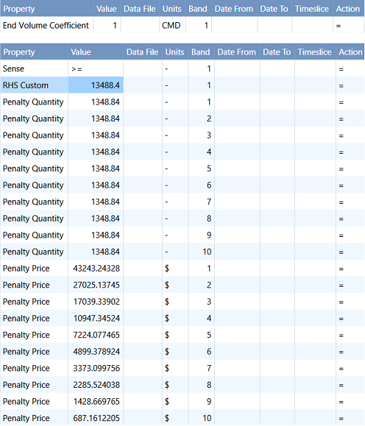 Figure 16: Water Value Constraint
RHS Custom is used so that only one constraint will be enforced at the end of horizon. The value of RHS Custom is equal to Max Volume of the storage, thus it defines a constraint as End Volume + Violation >= Max Volume, meaning that any water release (violation) bears a cost (penalty price), the more the released water, the higher the average cost. We used a penalty function of 10 bands in this example while any number of bands is allowed for defining the water value curve. Note that the End Effects Method should be set explicitly as Free when adding this water value constraint. One constraint should be defined for each storage.
6. Non-anticipativity Constraints
With all other constraints set, a Non-anticipativity constraint is introduced in stochastic optimization by setting property Trajectory Non-anticipativity and/or Generation Non-anticipativity to -1. This constraint is to restrict the variables (End Volume, Generation) across samples to be equal, meaning that only one set of decisions should be made today given the uncertain future.
7. Future Cost Function
The Future Cost Function (FCF) represents the future cost at different end volumes of storages, which is a multi-dimensional linear function with its slopes and intercept calculated in the deterministic solve (or called "pricing" step) at the end of rolling horizon. In this step we freeze the EndVolume solutions that recorded from each rolling and solve a deterministic optimization with periods spanning the entire horizon to get the shadow prices and the objective values. When both MT Schedule and ST Schedule are enabled, one FCF for each full branch will be produced in MT phase and it will be automatically passed to ST when Diagnostic Future Cost Function is selected, so that the shadow prices will be passed down to guide Storage Decomposition. The diagnostic file can be saved and used as an input for FCF to run ST Schedule alone without MT Schedule. Here is an example how it could be set via the Global Class:
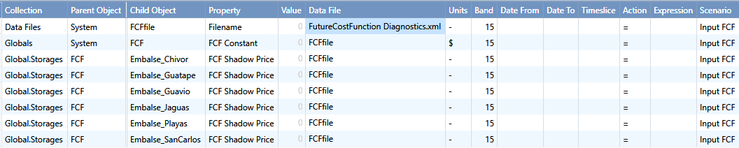 Figure 17: Enter FCF via Global
Non-physical inflows and spills required for feasibility.
8. References
- PARMA Parameter Estimation, S Ma, February 23, 2016.
- Stochastic streamflow model for hydroelectric systems using clustering techniques, D. Jardim, M. Macerira, D. Falcao, 2001 IEEE.