Unit Commitment
- Introduction
- The Unit Commitment Problem
- Mixed Integer Programming
- Rounded Relaxation Algorithm
- Dynamic Programming
- Stochastic Unit Commitment
1. Introduction
The term "unit commitment" refers to a sequence of generating unit on and off decisions made across time. The unit commitment "problem" is to find an optimal combination of these on/off decisions for all generating units across a given horizon. The on/off decisions must imply both a feasible solution and an optimal solution in terms of the total system cost including the cost of start up and shutdown. Unit commitment is part of the unit commitment and economic dispatch (UCED) algorithm, where economic dispatch refers to the optimization of generator dispatch levels for the given unit commitment solution. The UC and ED are co-optimized such that the combined costs of both UC elements, such as start costs, and dispatch costs such as fuel and O&M are minimized.
The constraints that apply exclusively to the unit commitment problem are:
Minimum Stable Level (MSL): The constraint that a unit must run at or above some minimum megawatt operating level in all hours that its commitment status is 'on'.
Minimum Up Time (MUT): The constraint that a unit must stay on for a minimum number of hours once it is started, unless it is interrupted by an unplanned outage.
Minimum Down Time (MDT): Likewise for number of hours the unit must stay off after being shut down.
Maximum Up Time: The (somewhat rare) constraint that a unit can only operate fora given number of hours after start up.
2. The Unit Commitment Problem
The difficulty in optimizing (and indeed in even finding a feasible solution for) generator unit commitment in a Linear Programming (LP) framework is that it involves integer on/off (1,0) decisions, and complex intertemporal constraints (MUT and MDT),neither of which cannot be directly solved by LP alone. However these problems can be solved by Mixed Integer Programming (MIP), sometimes referred to as Mixed Integer Linear Programming (MILP). In a MIP, certain variables are identified as being either binary (0,1) or general integers (taking any integer value) between specified bounds.
Commercial codes are available that solve MIP problems with reasonable efficiency, however MIP is much harder to solve than LP, and for large systems with thousands of generating units and a horizon of many days, weeks or years it might be impossible to solve the MIP directly.
Of course the simplest way to reduce the difficulty of the MIP is to not ask the simulator to make integer on/off decisions at all. By default the on/off decisions will be linearized, meaning that the LP may choose partial unit starts and shuts down. Linearization though has several side effects, including:
- Constraints involving integer decisions such as the MSL, MUT, and MDT cannot be enforced
- The shadow price on generator maximum capacity constraint will be influenced by any objective coefficients on the linearized on/off variable, which is equal to the no-load cost
- As a result the reported system λ (prices) will reflect average price at the marginal plant(s) rather than marginal cost
Note that in the simulation phases LT Plan and MT Schedule when the Chronology setting is "Partial" (the default) linearized unit commitment is employed. However, both phases provide options to switch between average cost and marginal cost pricing of generation (LT Plan Pricing Method, and MT Schedule Pricing Method).
For ST Schedule (always a chronological phase) you can switch the whole system to integer mode using the Production Unit Commitment Optimality setting, or individually using the property Generator Unit Commitment Optimality. However, if the optimal (or desired) unit commitment scheme for a generator is known a priori this pattern can be defined using the Generator Commit property. Pre-defining the commitment in this way not only reduces the size of the MIP but greatly simplifies the mathematical representation of the generator, so it is desirable to use the Generator Commit property wherever possible e.g. for any unit that must run in all periods where it is available, or that has a known on/off cycle. Note that Generator Commit only determines the UC solution for the Generator, the ED is still performed to find the optimal Generation.
The primary mechanism for reducing MIP complexity is to reduce the number of hours over which the MIP is solved i.e. by solving the planning horizon in multiple steps (solution of multiple small MIP being faster than one very large one). The Horizon settings provide exactly this functionality. For example a one year horizon can be divided into 365(6) daily steps, or in fact into any (equal-length) set of steps. Reducing the step size can have implications on the quality of the solution. A short step size (the shortest possible being controlled by Horizon Periods per Day) might be to short to properly optimize the UC with respect to the duration of MUT and/or MDT constraints. For example, dividing a year long simulation in to 8760 hourly steps is unlikely to yield an optimal UC for a unit with an eight hour MUT.
It's this scenario where the look-ahead functionality of ST Schedule is particularly useful. Look-ahead is the ability of each step to model an additional forward-looking period for the purpose of improving the UCED solution in the step. For example, one might run steps of 24-hour duration with an additional 6-hours of look-ahead. Step 1 then optimizes over 30 hours, but only keeps the first 24 hours of solution. Step 2 then picks up the initial conditions from hour 24 and solves again the next 30 hours, keeping the solution up to hour 48, and so on. Look-ahead is enabled with the Lookahead Indicator setting. To further improve performance, the Lookahead Periods per Day setting is allowed to set a lower resolution than the Horizon Periods per Day. For example, a one-hour step at 10-minute resolution could be supplemented with a 23-hour lookahead at hourly resolution. The total number of dispatch periods in a step is thus 29, rather than 144 if 10-minute resolution were used for the lookahead.
As alluded to above, reduction in MIP size (and therefore difficulty and solution time) can be achieved by reducing the resolution of the horizon from its default hourly setting e.g. solving with a time step of two hours should be more than twice as fast, at the cost of some accuracy in the averaging that will occur when hours are combined. This option is controlled by the Horizon Periods per Day setting.
Sometimes these reductions are either insufficient to gain acceptable performance, or are not suitable for the specific problem e.g. if some units have a minimum up or down time are very long. It is not uncommon in fact for large or particularly inflexible generating units to have minimum up and down times of more than two or even three days and if the system is very large it might not be feasible to use a long-enough step size. In this case an alternative strategy is needed - and two methods that can be used either separately or in combination are available. These are the Rounded Relaxation heuristic, and the Dynamic Programming optimization.
Firstly though, the mixed integer programming formulation and user settings are described.
3. Mixed Integer Programming
In this section we present elements of the mixed integer programming formulation for the UCED. The 'core' decision variable is the number of units operating in each dispatch period. This variable is given the symbol Ont, where t indexes time periods in chronological order t = 1, ... ,T. The economic dispatch variable is Loadt being the generation. Startt is the binary decision variable that indicates a unit has started in period t.
For clarity, in this document we assume each dispatch period is one hour, and we omit starting conditions or issues related to joining one simulation step to another. We also omit the index of generating unit and assume a single-unit generator. For multi-unit generators the constraints are in general repeated for each unit, except those that can be simplified to apply across all units.
3.1. Start, Stop and Commitment Logic
Loadt is the instantaneous megawatt generation of the unit at the end of period t, thus if Startt is one, then the unit is 'on' for the entire duration of period t, and thus Ont' must logically be one. In some cases the complementary variable Stopt is included in this formulation, and the logic for this variable is similar in that we have:
Ont = On(t-1) + Startt - Stopt ∀ t
In the absence of Stopt we must enforce that:
Ont ≥ Startt ∀ t
and:
Startt ≤ 1 - On(t-1) ∀ t
These last two constraints might seem redundant, but will bind in cases where a start is desirable ahead of the 'on' state, such as can occur when modelling Reserve in combination with ramp constraints. Note that these constraints can be either included 'upfront' in the formulation or added incrementally as required. The latter might provide a performance improvement, and this feature is accessed through the Production Formulate Upfront setting.
Start and shutdown costs require the respective variables to be included. When defined, these costs enter the minimization objective function with as follows:
Objective (Minimize):
StartCostt x Startt + ShutdownCostt x Stopt ∀ t
Note that start cost can vary according to the cooling state of the unit, and this requires additional complexity in the formulation, which we will not cover here. Further, start cost can include the cost of fuel used to start as defined by the Generator Start Fuels Offtake at Start property.
3.2. Minimum Stable Level
We denote the minimum stable level as MSL. The following constraint enforces the MSL in the MIP:
MSLt:
Loadt ≥ MSLt x Ont ∀ t
3.3. Minimum Up Time
We denote the minimum up time as MUT. The following constraints, generally referred to as "turn on" constraints, enforce unit minimum up time in the mixed integer program.
TurnOnt
Ont ≥ Startk ∀ t,k=t-1,t-MUT+1''
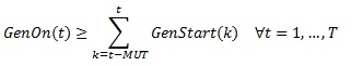
This equation set forces the status of the generating unit (represented by variable Ont) to be greater than zero if there is a start-up in any previous period in the scope of the Min Up Time. Note that this formulation requires the definition of Startt variables even if Start Cost is not defined or is zero.
3.4. Minimum Down Time
We denote the minimum down time as MDT. The following constraints, generally referred to as "turn off" constraints, enforce unit minimum down time in the mixed integer program.
TurnOfft
Ont ≤ 1 - Stopk ∀ t,k=t-1,t-MDT+1''
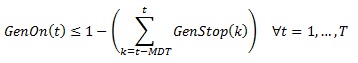
MDT constraints force the 'on' variable to be less than unity if there any of the Stopt variables are activated (1) in any of previous periods in the scope of the Min Down Time. Note that this formulation requires the definition of Stopt variables even if Shutdown Cost is not defined or is zero.
3.5. Solving the UCED Problem
MIP solvers are based on the Branch and Bound algorithm, complemented by heuristics designed to reduce the search space without comprising solution quality. Branch and Bound does not have predicable run time like linear programming. It is difficult in all but trivial cases to prove optimality and guarantee that the integer-optimal solution is found. Instead the algorithm relies on a number of stopping criteria that can be user defined. These criteria are exposed via the Performance object. The primary stopping options are the MIP Relative Gap and MIP Max Time.
Branch and Bound begins by solving the 'root node', which is a version of the linear relaxation i.e. the UCED problem with integer constraints relaxed, augmented with 'cuts' (constraints) that reduce the number of feasible integer solutions without excluding the optimal solution. Following this, the solver will perform heuristic operations such as a 'local search' in an attempt to find a high quality initial integer solution and/or to exclude as many solutions as possible, thus raising the objective value of the linear relaxation. The value of this 'worst' linear relaxation problem, that is known to still contain the optimal integer solution, is called the 'lower bound'. Proof of integer optimality is when the lower bound is within a tolerance of the objective function value of the best known integer solution. The difference between these objective values (the lower bound, and best integer) is referred to as the 'gap' as is usually expressed as a percentage computed as follows:
Gap = (BestIntegerSolution - BestBound) × 100 / BestIntegerSolution
For example, if the best integer solution found so far has an objective function value of 100 and the lower bound (worst linear solution that can still contain the integer optimal solution) is 99.9, then the gap is (100 - 99.9) × 100 / 100 = 0.1%. Note that the gap is not a measure of optimality, but rather an 'optimality proof'. In this example the best integer solution might actually be optimal, it is just that the lower bound has not been raised sufficiently to prove it, and likewise the best integer solution might be very close to the current lower bound. All that can be said is that the best integer solution can be no better than the lower bound, and no worse than the best integer solution.
It is highly desirable to find a good integer solution at the root node through heuristics and/or to raise the lower bound to a point that the Branch and Bound tree need only check a relatively small number of nodes. If optimality cannot be proven at the root node, the tree search starts. Depending on the solver and settings, further heuristic algorithm passes might be invoked at times during the tree search. The tree search terminates once optimality is proven according to the user-defined acceptable gap, or the time limit is reached. In rare cases, the Branch and Bound might consume so much memory in the tree search that system resources are exhausted.
A wide range of commercial third-party MIP solvers are supported. You select these with the Performance SOLVER setting. The solvers can vary considerably in their solution speed, depending on the particular dataset and stopping criteria used. Solution speed in MIP is a function of:
- The speed of the linear programming solver used to solve the root node, and each node of the Branch and Bound tree. Since the root node is linear, and each node of the tree search has integers fixed at some candidate values, all solve operations in the Branch and Bound are linear and thus raw linear programming speed is crucial.
- The quality of the cuts introduced at the root node, and of the root node heuristics. This can be a major differentiator between solvers, since solving at the root node and avoiding the tree search is a 'best case scenario'.
- Tree search rules and the quality and frequency of heuristics used at tree nodes. Exploring nodes seeks not only to find better integer solutions but also to raise the lower bound. The better the solver is at producing cuts that raise the lower bound, the faster it will reach an acceptable gap.
All the supported solvers have unique settings that control fine aspects of Branch and Bound. These solver-specific settings can be accessed via the Solver Parameters File if required.
4. Rounded Relaxation Algorithm
The Rounded Relaxation ("RR" for short) is a heuristic that aims to produce a feasible and high quality unit commitment solution without the need to run "full" mixed integer programming. The RR algorithm is invoked via the global setting Production Unit Commitment Optimality.
The RR works by rounding the linear relaxation unit commitment solution to the "nearest" integer values, while enforcing the MUT, MDT, and MSL constraints. Because of the need to enforce MUT and MDT, the algorithm is more complex than a simple rounding of individual hourly on/off decisions. In addition, the algorithm seeks to preserve as closely as possible the total commitment MW capacity in each region (as compared to the linearized solution). It uses multiple linear passes as well as decomposition similar to Lagrangian Relaxation.
The RR algorithm is fast, usually no more than doubling the run time of the linearized unit commitment. The Production Rounding Up Threshold controls how likely the algorithm is to round up a non-integer value. It may require some experimentation to find a 'best' value for this parameter and thus the additional option Production Rounded Relaxation Tuning allows you to turn on 'auto-tuning' of this parameter. Running the self-tuning RR takes more time, but will usually yield superior results.
5. Dynamic Programming
Dynamic programming (DP) is a technique that is well suited to the unit commitment problem because it directly resolves the MUT, MDT, and MUT constraints, and over long horizons. Its weakness is in the way unit commit is decomposed so that units are dispatched individually. Thus if all units in the system were dispatched using dynamic programming it would be difficult to converge on a solution where system-wide demand was met exactly, and where any other system-wide or group constraint such as fuel or emission limits were obeyed. For certain class of generator though DP can be fast and highly effective.
The DP is most suited to units with a high capacity factor, and if applied to all units in the system is likely to produce significant under/over generation. Thus you must carefully select units for which the DP is applied e.g. high capacity factor plant with long MUT or MDT values are most suitable.
DP can be invoked on selected generators by setting the property Generator Unit Commitment Optimality = "Dynamic Program". Generators selected for DP commitment have their unit commitment optimized in a stage between MT Schedule and ST Schedule. Thus you must enable MT Schedule for this to work.
Units selected for DP enter ST Schedule automatically with a strict Commit schedule representing the optimal unit commitment found by the DP. Thus in ST Schedule these generators have a simplified representation, which results in a faster solve and no need for integer elements for those generators. Thus DP can produce significant run time improvements in ST Schedule.
6. Stochastic unit Commitment
6.1. Uncertainty and Sampling
Stochastic unit commitment (SUC) refers to the optimization of unit commitment decisions under uncertainty. The uncertainty is typically in inputs such as the load, renewable generation (particularly wind and solar production) and outages although practically any input can be involved. SUC can be performed in any simulation phase but is typically modelled in ST Schedule. To enable SUC, first the simulation phase must be running in stochastic mode. For ST Schedule the setting Stochastic Method is set to "Scenario-wise Decomposition" to invoke this mode.
The uncertain variables are then defined via Variable objects e.g. to define stochastic series for Region Load for load, or Generator Rating for wind generation, or Storage Natural Inflow for inflows. The number of samples produced is controlled by the Stochastic Risk Sample Count and optionally reduced to a smaller set for simulation with the Reduced Sample Count setting.
6.2. Stochastic Optimization
The basic concept of SUC is that certain unit commitment decisions, such as the start up and shutdown of large, inflexible thermal plant must be made 'upfront' without fully knowing the outcome of the uncertain variables. Once those 'non-anticipative' decisions are made, the uncertain parameters are realized and we may make recourse decisions, such as dispatch or unit commitment decisions. The optimization then is over the set of non-anticipative unit commitment decisions plus the recourse decisions. The objective function minimizes the net present value of the expected total system cost i.e. the cost of all non-anticipative UCED decisions plus recourse decisions. The result is a set of unit commitment decisions that are non-anticipative (absent of the bias of perfect foresight) and robust (minimizing the expected cost given all modelled future outcomes and their probabilities and optimal recourse decisions).
This stochastic optimization is by default 2-stage, meaning that there is just one set of non-anticipative decisions (stage 1) and one set of recourse decisions (stage 2). The problem can be made multi-stage (3 or more stages) through properties of the Global object.
The following inputs define a 3-stage scenario tree with the first stage ending at interval 6, the second at interval 12 and the last running to the end of the step. If this were combined with Stochastic Risk Sample Count = 100, and Reduced Sample Count = 20, then the last stage will have 20 nodes, while stages one and two have 2 and 10 nodes respectively.
| Global | Property | Value | Units | Band |
|---|---|---|---|---|
| Tree | Tree Stage Count | 3 | - | 1 |
| Tree | Tree Stages Position | 6 | - | 1 |
| Tree | Tree Stages Position | 12 | - | 2 |
| Tree | Tree Stages Leaves | 2 | - | 1 |
| Tree | Tree Stages Leaves | 10 | - | 2 |
Refer to the Variable topic for more information about multi-stage stochastic optimization.
6.3. Non-anticipative Decisions
There are several UCED decision variables that can be nominated as 'non anticipative' and for all variables you choose the set of Generator that are subject to this constraint simply by setting properties on individual objects.
The properties for non-anticipativity work in pairs. The first property is a penalty value for anticipation, where a value of -1 means "infinity". The second property is a timeframe in hours over which the non-anticipativity constraints are enforced. The available pairs are:
- Generator Unit Commitment Non-anticipativity and Unit Commitment Non-anticipativity Time
- Generator Pump Unit Commitment Non-anticipativity and Pump Unit Commitment Non-anticipativity Time
- Generator Generation Non-anticipativity and Generation Non-anticipativity Time
- Generator Pump Load Non-anticipativity and Pump Load Non-anticipativity Time
In the following example a simple generation option can be purchased, but the decision to exercise the option must be made at the start of the day.
| Generator | Property | Value | Units | Band |
|---|---|---|---|---|
| OPTION | Unit Commitment Optimality | "Integer" | - | 1 |
| OPTION | Units | 10 | - | 1 |
| OPTION | Max Capacity | 10 | MW | 1 |
| OPTION | Min Stable Factor | 75 | % | 1 |
| OPTION | Unit Commitment Non-anticipativity | -1 | $ | 1 |
| OPTION | Unit Commitment Non-anticipativity Time | 24 | hrs | 1 |
| OPTION | Offer Quantity | 10 | MW | 1 |
| OPTION | Offer Price | 59 | $/MWh | 1 |
The following examples is of a demand-side option modelled as a pumped storage. Here, both the generation and pump load side of the option are subject to non-anticipativity constraints.
| Generation | Property | Value | Units | Band |
|---|---|---|---|---|
| DR | Units | 1 | - | 1 |
| DR | Max Capacity | 10 | MW | 1 |
| DR | Min Stable Factor | 50 | % | 1 |
| DR | Pump Unit Commitment Non-anticipativity | -1 | $ | 1 |
| DR | Pump Unit Commitment Non-anticipativity Time | 24 | hrs | 1 |
| DR | Generation Non-anticipativity | -1 | $ | 1 |
| DR | Generation Non-anticipativity Time | 24 | hrs | 1 |
| DR | Pump Efficiency | 90 | % | 1 |
| DR | Pump Load | 12 | MW | 1 |
| DR | Min Pump Load | 12 | MW | 1 |
6.4. Stochastic Solution
Having nominated the non-anticipative decisions the SUC is solved in the simulation. What characterizes the SUC solution over its perfect-foresight equivalent is that the optimal value of the those decisions across all samples will be identical over the time period of non-anticipativity. In addition it is expected that the objective function value of the SUC is higher (more costly) than the weighted sum of objectives of the perfect foresight independent sample solutions. However, if the optimal non-anticipative decisions are applied to the independent samples e.g. if you feed those unit commitment solutions to the independent samples, the resulting costs are better than any other non-anticipative solution, for example, better than simply taking the average of the unit commitment solutions from the independent samples.
6.5. Interleaved Mode
Model Interleaved goes hand-in-hand with SUC. For example to simulate a day-ahead unit commitment followed by a real-time 'realization' you can use a stochastic unit commitment in the master model "Day Ahead" and interleave this with a second Model "Real Time" running with either a single or multiple realizations in independent samples mode. See the Model topic for more information on interleaved mode.
6.6. Forecast Timeframes
When modelling with Interleaved and in some other circumstances you might need to change the forecast values applied in each simulation step depending on the hour of the step. For example, in a day-ahead simulation with a 24 hour step plus another 24 hours look-ahead the first 24 hours will have a more accurate forecast of load, etc than the hours 24-48. These two forecasts can be input on Variable objects and defined with properties as in the following example.
ExampleThe Variable objects are defined as active but with a period range 1-24 for "Intra-day" and 25-onwards for "Day-ahead".
| Condition | Property | Value | Units |
|---|---|---|---|
| Day-ahead | Include in LT Plan | 0 | Yes/No |
| Day-ahead | Include in PASA | 0 | Yes/No |
| Day-ahead | Include in MT Schedule | 0 | Yes/No |
| Day-ahead | Include in ST Schedule | -1 | Yes/No |
| Day-ahead | Step Hour Active From | 25 | - |
| Day-ahead | Step Hours Active | -1 | - |
| Intra-day | Include in LT Plan | 0 | Yes/No |
| Intra-day | Include in PASA | 0 | Yes/No |
| Intra-day | Include in MT Schedule | 0 | Yes/No |
| Intra-day | Include in ST Schedule | -1 | Yes/No |
| Intra-day | Step Hour Active From | 1 | - |
| Intra-day | Step Hours Active | 24 | - |
These conditions are then applied to the Variable tags for the forecast related properties.
| Region | Property | Value | Units | Band | Date From | Date To | Timeslice | Condition | Variable |
|---|---|---|---|---|---|---|---|---|---|
| A | Load | 0 | MW | 1 | Day-ahead | Day-ahead Forecast Load | |||
| A | Load | 0 | MW | 1 | Intra-day | Intra-day Forecast Load |