Portfolio Optimization

Aurora can perform portfolio optimization using a risk-reward framework and a linear optimization model. Use this capability to lay out the mathematical framework under which the optimization operates.

The goal of the optimization is to calculate a number of optimal portfolios—those with the highest reward and lowest risk—given the constraints of the portfolio and its acquirable resources. Each portfolio found by the simulation will lie along the Efficient Frontier, which means that no other portfolio with higher reward at the same risk level exists, and no other portfolio with lower risk at the same reward level exists. The final result of the optimization will produce a set of one or more portfolios along this risk/reward frontier:

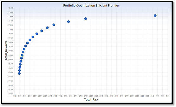
Each of these points on the chart represents a portfolio of acquired resources with their imputed costs, generation, etc. This set of resources with their forecasted operational data then implies the market purchases and sales, reserve margin, RPS level, and other portfolio characteristics of the time frame being considered.

The cost and generation of resources is derived from the reported data from standard Aurora risk simulations which are performed previous to the optimization. In other words, the output data from standard Aurora runs becomes the input data to the optimization. This output data is processed by the optimization in order for the model to calculate expected values for generation and costs of potential portfolio resources for each time period, as well as expected market prices and portfolio demand. The optimization estimates the portfolio variance—the risk measure—based on the resource operation under the iterative risk scenarios in the output.

The portfolio optimization capability in Aurora provides a flexible tool for evaluating the performance of resources under a wide range of future scenarios. It joins the LT Capacity Expansion and Monte Carlo Risk capabilities in the model to offer a mathematically rigorous method for determining the best future portfolios for a given entity. The rest of this document describes in detail how to use the functionality as well as the mathematical formulation behind the optimization.

Initial Simulations

Running Risk Scenarios

One of the first steps in the portfolio optimization setup is to decide which resources and contracts are available to be acquired. These options can exist directly in the Resources or Portfolio Contracts table, and they can also come from an RMT table resulting from a long-term study. For example, a user might run a long-term study to let the model decide which resources (system wide) are most likely to be built and then select which of those resources are potential candidates for their portfolio. Or a user may want to simply define a set of candidate resources in the Resources table which are believed to be available in the future. Portfolio contracts can be defined as well to provide options to the portfolio which do not affect market prices in the standard simulations.

Once the resources and contracts are selected, standard Aurora simulations need to be run with output being reported for each of these options. All of these are performed prior to actually running the portfolio optimization capability. If only the least cost portfolio is of interest to the user, then one such standard simulation is adequate, but to calculate the portfolio risk multiple runs are required. Generally for the most robust solution, numerous risk simulations should be completed so that the candidate resources’ performance can be seen under many different future scenarios. There is no maximum number of risk runs that can be read in by the optimization, but all iterations must exist in the same output database.

A user may also choose to run multiple long-term simulations in the model, each with a different future scenario (e.g. low gas price case, medium gas price case, and high gas price case). Each of these long-term runs would produce a unique RMT table with potentially overlapping new resources which the long-term logic chose to build. A set of candidate resources for the optimization could then be selected from the union of all new resources in the RMT tables, and some number of risk runs could be performed for each RMT table. The total set of all those risk runs could then become the basis for the optimization. Using this setup, it is likely that some candidate resources would not exist in all of the output iterations (e.g. the resource was built in one long-term scenario but not in another). For those iterations the optimization would assume zero cost and zero generation for that resource.

NOTE: When using this multi-RMT approach, the impact of each original long-term case on the optimization will be weighted by the number of risk runs each RMT is used in.

Care should be taken in deciding which inputs will be randomly adjusted during these pre-optimization simulations so as not to bias one portfolio resource option over another. Which of these input values will be shocked in the risk simulations is completely defined by the user. The internal Aurora risk logic can be used to automatically adjust inputs such as demand, fuel prices, hydro capability, transmission link availability, resource outages, and portfolio demand. If the user prefers to feed in random draws from outside of Aurora, this can likewise be done using the scripting or CDS capabilities in the model. Each separate run performed will receive an equal weighting by the optimization as it evaluates the projected value of each resource and contract. The portfolio optimization will distinguish risk iterations in the output by either using the Risk_Iteration or Run_ID output column, as defined by the Output Identifier on the Simulation Options form.

Selecting the Optimization Time Period

The available time periods by which the output data can be divided for the optimization are Hour, Day, Month, and Year. Each of the time periods except for Hour can be further subdivided into two or more conditions. The optimization will take the output data for each “time bucket” (a specific condition within a specific time period) and guarantee that the constraints are met. For example, suppose a user wanted to run the optimization over a ten year window with two conditions, on-peak and off-peak. If the Time Period selected was Year, then the model would divide the data into twenty time buckets (on-peak and off-peak for each year) and ensure that the demand and market purchases/sales constraints were met for those time buckets. If the Time Period selected was Month, the model would divide the data into 240 time buckets (two in each month) and ensure that the monthly demand and market constraints were met for each of those month-condition buckets. The more granular this Time Period selection, the longer the run time of the actual optimization will be.

NOTE: While there is no specific limit on the number of conditions which can be specified (except for the Hour time period which can only have one), the conditions should exactly cover a full week. Conditions in Aurora are defined using a 168-hour vector, so the conditions used for the optimization should completely specify all 168 hours, and no hour should be in multiple conditions. The optimization sums up the reported numbers for each time bucket into annual values—needed for the RPS and Reserve Margin constraints—and so it assumes that the conditions are non-overlapping and cover a full week.

Reporting Needed for the Optimization

During the simulations which are run before the optimization, a standard portfolio with associated demand must be set up in the Portfolio Information table.This demand will be used as the demand for the optimization and can be adjusted automatically by the Aurora risk logic. In the Portfolio folder of Simulation Options, the first two Portfolio Settings should be selected (Run portfolio analysis and Use market sales and purchases). This portfolio does not need to have any associated contracts or resources.

In addition, during the risk runs the following output tables need to be reported for the Time Period (Year, Month, Day, or Hour) selected in the optimization:

Resource
Zone
PortfolioSummary
PortfolioContracts (if portfolio contracts are being used)

For these tables above, all specified conditions for the optimization should be selected to be written to the output.

NOTE: The PortfolioSummaryYear and ZoneYear output tables must also be reported, regardless of the optimization Time Period. Both the optimization conditions and the Average condition should be written for these two tables.

If Custom Column reporting is being used to trim down the output database size, the following columns must be selected for all of the required output tables:

Study_Info
Report_Year
Condition
Time_Period
Run_ID
Risk_Iteration

In addition, the following columns are needed for each individual output table:

Resource: ID, Report_Level, Beg_Date, End_Date, Capacity, Output_MWh, Total_Fuel_Cost, Variable_OM_Cost, Total_Emission_Cost, Startup_Cost, Fixed_Cost, Fixed_Cost_Base, Fixed_Cost_Aux1, and Fixed_Cost_Aux2
Zone: ID, Price, Demand, Demand_Total, and Capacity_Credit
PortfolioSummary: Portfolio_ID, Portfolio_Demand_Total, Act_Max_Portfolio_Demand, and Act_Max_Portfolio_Date
PortfolioContracts: Contract_Number, Contract_Energy_Total, and Contract_Cost_Total

NPV Calculations

In the standard Aurora simulations, all financial values are reported in currency for some specific year as labeled in the Study_Info column of all output tables. When the optimization reads in any needed financial values, it will also determine what year the currency data is in. The simulation will subsequently convert that financial data into a net present value (NPV) in terms of the start year of the optimization (as specified in the Period/Hours folder of the Simulation Options form). To do this, the model will first use the standard inflation vector in the Time Series Annual table to convert values into currency of the optimization start year. The Real Discount Rate, found in the input General Information table, will then be used to discount the values back to the start year. All financial data used in calculations in the optimization will be NPV values, and all financial information in the optimization output tables will be reported in NPV terms.

Optimization Setup

Portfolio Optimization Input Table

Once the standard risk runs are completed, the optimization can be run. For this, the Portfolio Optimization input table must be populated to define the options available for acquisition in each portfolio:

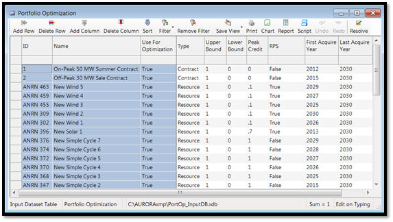
Each line in this table corresponds to exactly one resource or contract which should have operation data in the Resources or Portfolio Contracts output tables. In the optimization each of these options will be acquired at some level from 0% to 100%, and this can be further constrained using the Lower Bound and the Upper Bound columns. In these two columns an input value of 1 corresponds to acquiring the option at a level of 100%. For example, resources which must be part of the portfolio should have a Lower Bound and Upper Bound equal to 1. In this table the user also specifies the Peak Credit, which defines how much of each item’s capacity counts towards meeting the annual reserve margin. The RPS column allows each resource or contract to be specified as a renewable resource to define whether it contributes to meeting the input RPS target.

Optimization Constraints

The Portfolio Optimization form in Simulation Options must also be populated before running the optimization. In it the user can specify details about the portfolio optimization:

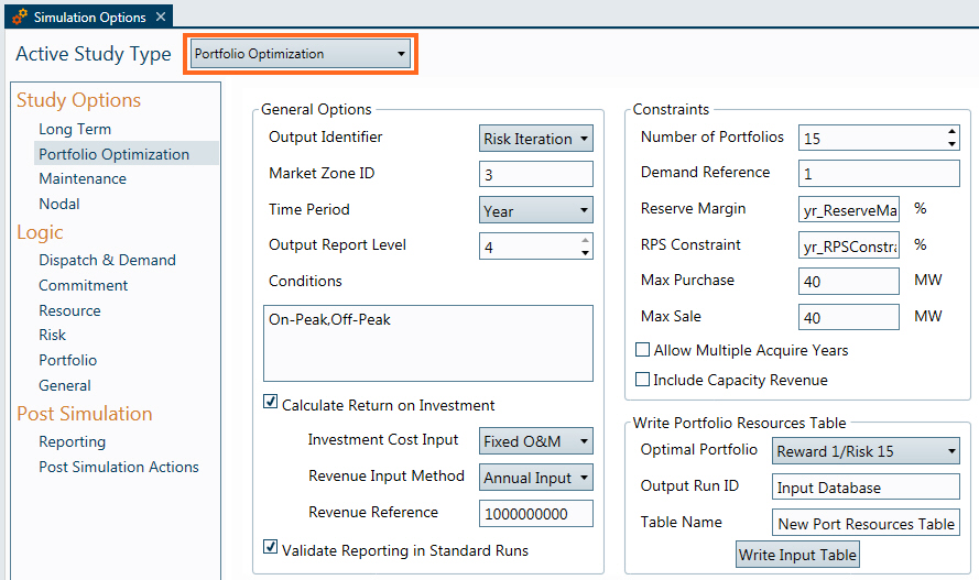
On the right-hand side of this form are the constraints which will be used in the optimization. These are the user-defined constraints for the optimization and how they are interpreted in the linear program:

Number of Portfolios: Defines how many portfolios on the efficient frontier the optimization will produce. An entry of 1 will calculate the least cost portfolio and ignore the risk metric. Otherwise, the optimization will calculate the least risk and least cost portfolios with the remaining number of portfolios in between along the efficient frontier.
Reserve Margin (%): An annual reserve margin target can be specified to ensure that an appropriate amount of capacity is acquired in the portfolio. This input value can be a constant or a reference to the Time Series Annual table. For each full year of output data, the optimization will be constrained such that

100*(1 - [Acquired Reliable Capacity]/[Peak Demand]) >= [Reserve Margin Target]

Note that the acquired capacity above will have been adjusted by the input peak credit values. The peak demand values are reported in the PortfolioSummaryYear output table. To make this constraint non-binding, the Reserve Margin Target should be set to -100. Optionally, this field can also specify a maximum constraint that the reserve margin cannot exceed entered as two inputs via a comma delimited list. For example, an entry could be "yr_MinReserveMargin, yr_MaxReserveMargin".

RPS Constraint (%): An annual RPS constraint can also be entered for the portfolio to ensure that an adequate amount of renewable generation is acquired for the portfolio. The model will ensure that for each year

[RPS Resource Generation (MWh)] >= [RPS Percent] * [Annual Demand (MWh)]

To disable this constraint, the RPS Percent value should be set at 0. Optionally, this field can also specify a maximum constraint that RPS generation cannot exceed and is entered as two inputs via a comma delimited list. For example, an entry could be "yr_MinRPS, yr_MaxRPS".

Market Purchases/Sales Constraint: The optimization will ensure that for each time bucket the portfolio does not exceed the input market sales and purchases constraints. These two input values are entered as a MW amount and converted internally into a MWh number for each time bucket. For example, if a value of 100 MW is entered as the max purchase value and a certain time bucket contains 440 hours, the linear program will be constrained such that the total market purchases for that period does not exceed 44000 MWh.
Allow Multiple Acquire Years: This setting determines whether resources and contracts can be acquired at years later than their begin dates. Without this selected, the model will require that if a resource or contract is acquired at any level, it must enter the portfolio on its begin date or the first year of the optimization (whichever comes later). The resource or contract will subsequently remain in the portfolio throughout the duration of the study horizon at the same constant level of acquirement. If this switch is checked, on the other hand, then the model will be permitted to acquire resources and contracts during some range of years as input by the user. For example, the model might choose to acquire a resource at 25% in one year, and then acquire 20% more of that resource in some later year. The range of years for which an item can be acquired is specified using the Portfolio Optimization table.

NOTE: The Lower Bound constraint for a particular option will be honored as of the last acquirable year for that item. Also note that using this selection can greatly increase the run time of the optimization. When allowing this option, users should limit the range of years for each resource or contract as much as possible to ensure the fastest run times.

Include Capacity Revenue: This switch determines whether capacity revenue and the cost of capacity demand will be accounted for in the optimization. If selected, the capacity revenue for each resource will be a part of the total portfolio cost calculation. A capacity cost will also be calculated based on the annual peak demand and the capacity prices. Each portfolio will incur an annual cost equal to [Annual Capacity Price ($/MW/yr)]*[Peak Demand]. If this switch is not selected, it will be assumed that no resources receive revenue for capacity and that the portfolio does not have any capacity costs to pay.

Calculating Return on Investment

On the Simulation Options form the user also has the option to specify whether the optimization will report information about the return on investment for the portfolios. If the Calculate Return on Investment switch is selected, the optimization will perform additional post processing to report the expected revenue and return on investment for the portfolios. The linear program will minimize the total portfolio cost, after which the revenue data will be added to calculate an expected reward for the portfolio. The revenue is an extra input into the simulation and can be entered by the user in one of three ways:

Annual Input: An annual amount (in real base year currency) is input either as a fixed value or in a Time Series Annual reference.
Annual Price: An annual price (in real base year currency) is input either as a fixed value or in a Time Series Annual reference. This value is multiplied by the expected annual demand for each year to get the total annual revenue.
Market Price: The average market price for each year is multiplied by the expected annual demand for each year to get the total annual revenue. If Include Capacity Revenue is selected, then the capacity price (converted to a currency/MWh value) is added to the annual energy price.

From these input values, the model will calculate a total expected revenue for the portfolios over all the years of the study. This value will be the same for all portfolios along the efficient frontier in the optimization. Based on what resources are acquired in each portfolio, the model will also calculate an expected investment cost. This will come from the column specified by the Investment Cost Input selection on the Simulation Options form. Based on those two values—total reward and total investment cost—a return on investment will be calculated using a standard IRR-style approach. This value for each portfolio will be reported in the PortOp_EfficientFrontier output table.

NOTE: The use of the Calculate Return on Investment switch will not change which resources are acquired in each portfolio.

Mathematical Framework (Risk Metric = Variance)

This next section describes the mathematical framework for the optimization in greater detail. It lays out how portfolio cost and risk are defined and how the LPs are performed to find the portfolios along the efficient frontier. For the notation in this section, assume that the word “resource” refers to either an Aurora resource or portfolio contract, and that the term “time period” refers to a specific time bucket as already explained above.

Portfolio Notation

Assume the following general notation:

There exist r candidate portfolio resources over m time periods.
For a portfolio selected from the set of r resources, the proportion of resource j held in the portfolio is denoted a_j. In this context, each a_j must lie in the unit interval, i.e., .
a is the column vector (a₁, a₂, … , a_r)'.
I is an identity matrix, with dimension indicated by context.
E_αβ is an α by β array of 1s.

From each individual Aurora simulation, assume the following notation:

In time period i, resource j has a total cost C_ij. This includes fuel costs, emissions costs, variable O&M costs, startup costs, and fixed costs.
Resource j may also have capacity revenue in period i, denoted as RK_ij.
The energy generated in period i by resource j is denoted G_ij.
Portfolio demand in period i is denoted D_i.
Portfolio capacity demand (annual peak demand) in year y is denoted DK_y.
Average market price in period i is denoted p_i.
Average capacity price in year y is denoted PK_y.
Denote the following arrays:
- RK is an m by r matrix, {RK_ij}.
- G is an m by r matrix, {G_ij}.
- p is the column vector (p₁, p₂, … , p_m)'.
- PK is the column vector (PK₁, PK₂, … , PK_m)'.
- D is the column vector (D₁, D₂, … , D_m)'.
- DK is the column vector (DK₁, DK₂, … , DK_m)'.

With this notation, a portfolio is a triplet of values for the vectors a, D and DK. For Aurora portfolio optimization, a is the only one of the three variables subject to adjustment, D and DK being fixed (as calculated from the output data). Thus a becomes the vector of decision variables which will ultimately be solved for by the linear program when each portfolio is derived.

Defining Portfolio Cost and Variance

The total net cost of a portfolio in a run can be defined as the sum of four parts:

The cost of holding shares of resources held in the portfolio:
The cost of market transactions required to balance the portfolio demand with the energy production of the resource shares held in the portfolio:
Optionally, if capacity prices and revenues are used, the cost of capacity corresponding to the portfolio demand:
Optionally, if capacity prices and revenues are used, the negative capacity revenues from shares of resources held in the portfolio:

Thus the net portfolio cost B is:

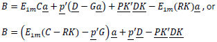
Define the vector NC’ as 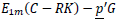, and the final cost equation becomes

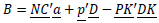
There are three terms on the right side of this equation, only one of which involves a. To simplify the relevant algebra, write the three terms as:

Then the total portfolio cost can be written as:

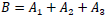
The total portfolio variance can be written as Var(B) =

Optimization Objective Functions

The optimization will use both cost and variance as objective functions for the linear program, so we need to be able to formulate both of these as a linear function of the decision variables vector a.

To do this for portfolio cost, we need to find the expected values which make up equation 1. The total expected portfolio cost becomes:

All the expected values in this expression are estimated by taking averages of the terms in brackets across the set of underlying Aurora runs. Note that when only one run has been performed, these expected value terms are simply the values from that run.

To describe the total portfolio variance as a linear function of a, we can expand equation 2 as follows:

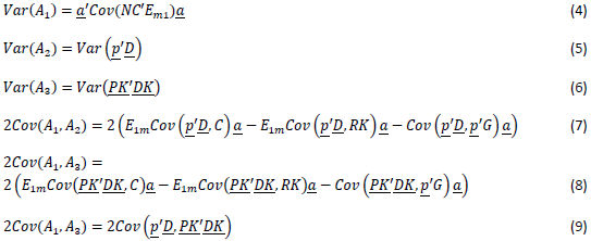
The estimated variance of a scalar, such as in equations 5 and 6 above, is the sample variance of its value over the underlying Aurora runs. When vectors appear in the Cov() notation, the result is the estimated covariance matrix found by using the iterative data from the underlying Aurora runs. When two different arguments appear in Cov(), the implied covariance matrix will be d₁-by-d₂, where d₁ is the length of the first vector argument, and d₂ the length of the second. When the variance values are calculated, the unbiased sample estimate is always used.

Equation 4 is in a quadratic form which must be further transformed as a linear function of new decision variables. A linear approximation method using matrix diagonalization as well as a concept known as the principle of adjacent weights is used to be able to express Var(A1) as a linear function of a and other newly defined decision variables. The details of this technique are not delineated here. Testing has shown that the approximation technique used generally differs by less than .01% from the actual quadratic variance calculation.

Simulation Sequence

Once the output data has been processed and the cost and variance information has been set up, this is how the simulation proceeds to find the optimal portfolios:

First the least cost portfolio is determined by having portfolio cost as the objective function to be minimized with no constraint on the portfolio risk. Once the LP solves, the total cost and total risk values are determined, and this becomes the first end point of the efficient frontier.
If only one portfolio is requested by the user (as specified in the Number of Portfolios entry on the Simulation Options form), then no more portfolios will be found. Otherwise, the least risk portfolio is then found by having the risk value as the objective function to be minimized with no constraint on the portfolio cost. The total cost and total risk values are determined, and this becomes the second end point of the efficient frontier.
If only two portfolios are requested by the user, then no more portfolios will be found. Otherwise, the model will find subsequent portfolios by setting the total cost to values equally spaced along the efficient frontier and minimizing risk at each of those cost levels. For example, suppose four portfolios were requested, the minimum risk portfolio had a cost of $1,750,000, and the minimum cost portfolio had a cost of $1,000,000. Two more portfolios would be needed, and their cost values would be set at $1,250,000 and $1,500,000. Two additional optimizations would be performed with risk as the objective function to minimize and with total cost constrained to be less than or equal to $1,250,000 and $1,500,000, respectively.
Once each portfolio along the efficient frontier is found, the reward and return on investment for each is calculated (if requested by the user). Detailed resource operation and costs, market sales and purchases, and overall portfolio statistics are likewise processed and reported in the output tables.

Output Reports

Summary Level Output

Two output tables will automatically be written with each portfolio optimization run: PortOp_EfficientFrontier and PortOp_ResourceAcquisition. They provide summary-level information about each optimal portfolio’s performance as well as overall statistics for each resource and contract in the optimization. The portfolios are automatically named by the model in the Optimal_Portfolio column with the convention Reward #/Risk #. For example, if 4 portfolios are requested by the user, then these will be named Reward 1/Risk 4, Reward 2/Risk 3, Reward 3/Risk 2, and “Reward 4/Risk 1. This nomenclature allows the user to see quickly where each portfolio ranks in terms of reward and risk among the others (e.g. Reward 2/Risk 3 has the 2nd best reward and the 3rd least risk of the portfolios found).

The PortOp_EfficientFrontier table reports one line for each optimal portfolio found. The total portfolio cost, along with each major cost component, is reported for every portfolio found by the optimization. In addition, the total demand, net market purchases, and resource generation is listed. The total risk value is reported as a standard deviation (square root of the variance), and the return on investment for each portfolio is reported if requested by the user. The format of the table allows for very easy charting.

The PortOp_ResourceAcquisition table lists how much each resource and contract was acquired in each of the optimal portfolios. Each candidate will be acquired at some level between its lower and upper bound as specified by the user in the input Portfolio Optimization table. If Allow Multiple Acquire Years is selected (in Simulation Options), then this table will show all of the potential years in which each option could have been acquired.

Detailed Reports

Three other output tables can be written after the optimization: PortOp_AnnualReport, PortOp_ResourceOperation, and PortOp_ResourceValidation. The first two give detailed information about the performance of each portfolio at more granular levels than the two summary output tables, whereas the PortOp_ResValidation gives information about resource options independent of any particular portfolio. The selection in the Output Report Level on the Simulation Options form determines which of these three tables will be written.

The total costs for each portfolio at an annual level can be found in the PortOp_AnnualReport output table. Information about yearly reserve margins, RPS percent, resource generation, market purchases, demand, and other information is also reported there. This is especially useful in validating that each portfolio meets the input reserve margin and RPS target specified by the user.

The PortOp_ResourceOperation table gives information about how each resource and contract operated within each optimal portfolio for each time period and condition. It also reports the information about the net market purchases (cost and energy) for each of the distinct time buckets for each portfolio.

Unlike the other four portfolio optimization output tables, the PortOp_ResourceValidation report does not give information about specific optimal portfolios. Instead it reports the expected operation data for each candidate resource and contract for each time period and condition. This allows the user to see the expected values for each portfolio option as they were calculated from the existing output database. These expected values are calculated as the average over all iterations in the output database, with financial data being adjusted to the NPV in terms of the start year of the optimization.

Conclusion

The portfolio optimization capability in Aurora provides a flexible and robust tool to model the risk and value of acquirable resources and contracts. When used in conjunction with the Monte Carlo Risk functionality and LT Capacity Expansion tools in the model, the optimization allows users to derive the highest reward portfolios under a standard Modern Portfolio Theory framework. Combined with Aurora’s easy data integration, detailed output reports, and automation tools, this capability provides a fast, mathematically sound methodology for modeling portfolio analysis and hedging against the uncertainty of the future.

Knowledge Base

Portfolio Optimization